Comparing with mean (with signal) Recover R=50
Yuxin Zou
2018-04-26
Last updated: 2018-05-17
Code version: 04f5122
Loading required package: ashrcorrplot 0.84 loaded#' Create simulation with signal
#' @param nsamp number of samples of each type
#' @param ncond number of conditions
#' @param err_sd the standard deviation of the errors
#' @details The simulation consists of equal numbers of four different types of deviations: null, equal among conditions, present only in first condition, independent across conditions
#' @export
sim.mean.sig = function(nsamp = 100, ncond = 5, R = 10, err_sd=sqrt(0.5)){
# generate scalar
Cs = rnorm(nsamp, R)
C = matrix(rep(Cs,R), nrow=nsamp, ncol=R)
# 90% null
nsamp.alt = ceiling(0.1*nsamp)
D.zero = matrix(0, nrow=nsamp-nsamp.alt, ncol=R)
# 10% alt
nsamp.all = floor(nsamp.alt)
# generate delta
D.all = matrix(0,nrow=nsamp.all, ncol=R)
d1 = rnorm(nsamp.all,sd=2)
D.all[,1:ncond] = matrix(rep(d1, ncond), nrow=nsamp.all, ncol=ncond)
D = rbind(D.zero, D.all)
C = C + D
Shat = matrix(err_sd, nrow=nrow(C), ncol=ncol(C))
E = matrix(rnorm(length(Shat), mean=0, sd=Shat), nrow=nrow(C),ncol=ncol(C))
Chat = C+E
row_ids = paste0("sample_", 1:nrow(C))
col_ids = paste0("condition_", 1:ncol(C))
rownames(C) = row_ids
colnames(C) = col_ids
rownames(Chat) = row_ids
colnames(Chat) = col_ids
rownames(Shat) = row_ids
colnames(Shat) = col_ids
return(list(C=C,Chat=Chat,Shat=Shat))
}The data contains 50 conditions with 10% non-null samples. For the non-null samples, it has equal effects in the first c conditions.
Let L be the contrast matrix that subtract mean from each sample.
\[\hat{\delta}_{j}|\delta_{j} \sim N(\delta_{j}, \frac{1}{2}LL')\] 90% of the true deviations are 0. 10% of the deviation \(\delta_{j}\) has correlation that the first c conditions are negatively correlated with the rest conditions.
We set \(c = 2\).
set.seed(1)
R = 50
C = 10
data = sim.mean.sig(nsamp=10000, ncond=C, R=R)
Discard last column
Mash contrast model
L = matrix(-1/R, R, R)
diag(L) = (R-1)/R
row.names(L) = colnames(data$Chat)
L.50 = L[1:(R-1),]
mash_data = mash_set_data(Bhat=data$Chat, Shat=data$Shat)
mash_data_L.50 = mash_set_data_contrast(mash_data, L.50)
U.c = cov_canonical(mash_data_L.50)
# data driven
# select max
m.1by1 = mash_1by1(mash_data_L.50)
strong = get_significant_results(m.1by1,0.05)
# center Z
mash_data_L.center = mash_data_L.50
mash_data_L.center$Bhat = mash_data_L.50$Bhat/mash_data_L.50$Shat # obtain z
mash_data_L.center$Shat = matrix(1, nrow(mash_data_L.50$Bhat),ncol(mash_data_L.50$Bhat))
mash_data_L.center$Bhat = apply(mash_data_L.center$Bhat, 2, function(x) x - mean(x))
U.pca = cov_pca(mash_data_L.center,2,strong)
U.ed = cov_ed(mash_data_L.center, U.pca, strong)
mashcontrast.model.50 = mash(mash_data_L.50, c(U.c, U.ed), algorithm.version = 'R', verbose = FALSE)Warning in REBayes::KWDual(A, rep(1, k), normalize(w), control = control): estimated mixing distribution has some negative values:
consider reducing rtolWarning in mixIP(matrix_lik = structure(c(0.143377883157803,
0.463026219647857, : Optimization step yields mixture weights that are
either too small, or negative; weights have been corrected and renormalized
after the optimization.Using mashcommonbaseline, there are 609 discoveries. The covariance structure found here is:
barplot(get_estimated_pi(mashcontrast.model.50),las = 2, cex.names = 0.7)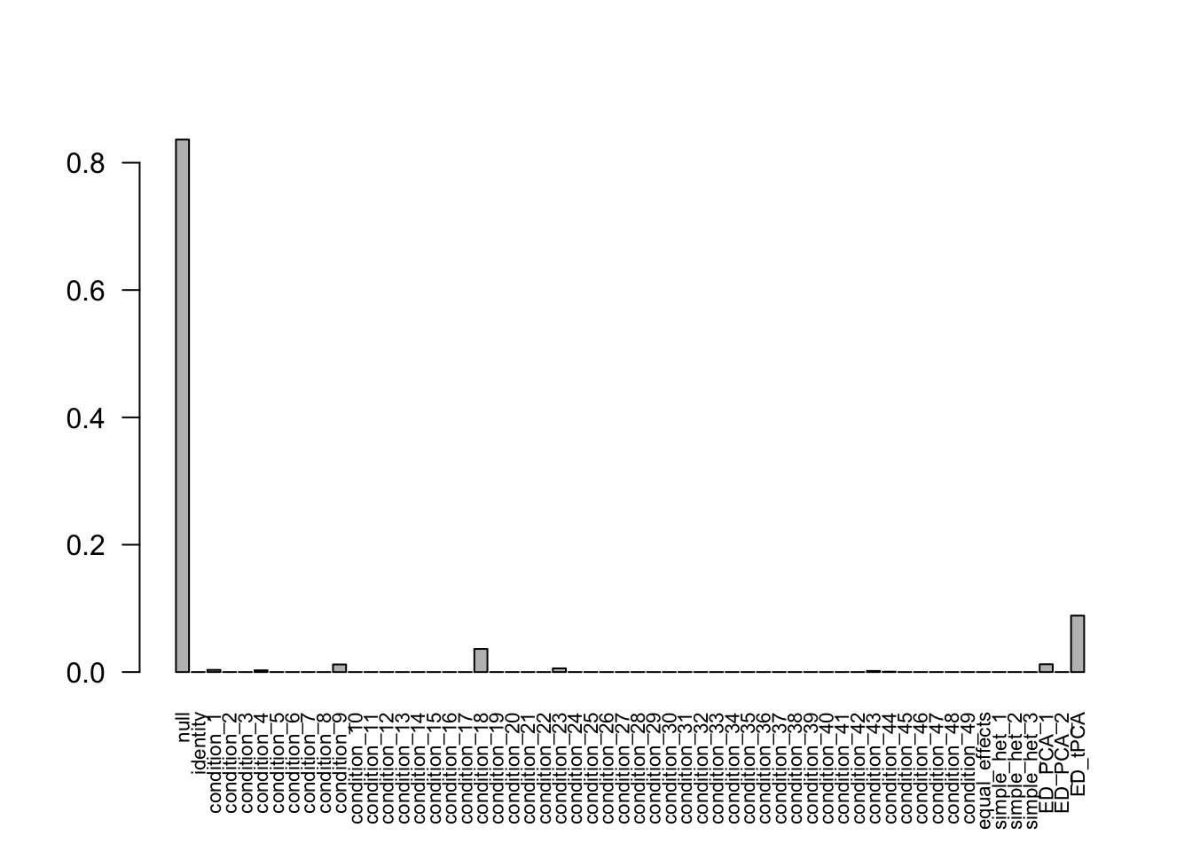 The correlation for tPCA is:
Recover the last column
mashcontrast.model.50.full = mashcontrast.model.50
mashcontrast.model.50.full$result = mash_compute_posterior_matrices(g = mashcontrast.model.50, data = mash_data_L.50, algorithm.version = 'R', recover=TRUE)
There are 610 discoveries.
Subtract mean directly
If we subtract the mean from the data directly \[Var(\hat{c}_{j,r}-\bar{\hat{c}_{j}}) = \frac{1}{2} - \frac{1}{2R}\]
Indep.data.50 = mash_set_data(Bhat = mash_data_L.50$Bhat,
                           Shat = matrix(sqrt(0.5-1/(2*R)), nrow(data$Chat), R-1))

Indep.model.50 = mash(Indep.data.50, c(U.c, U.ed), algorithm.version = 'R', verbose = FALSE)
Warning in REBayes::KWDual(A, rep(1, k), normalize(w), control = control): estimated mixing distribution has some negative values:
consider reducing rtolWarning in mixIP(matrix_lik = structure(c(0.00667820972445304,
0.0631737437819963, : Optimization step yields mixture weights that are
either too small, or negative; weights have been corrected and renormalized
after the optimization.There are 613 discoveries. The covariance structure found here is:
barplot(get_estimated_pi(Indep.model.50),las = 2, cex.names = 0.7)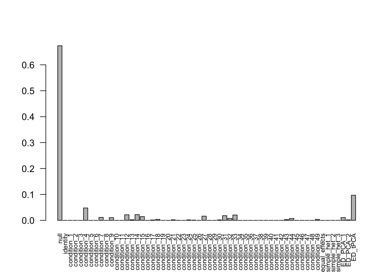
The correlation for tPCA is: 
Recover the last column
Indep.model.50.full = Indep.model.50
Indep.model.50.full$result = mash_compute_posterior_matrices(g = Indep.model.50, data = Indep.data.50, algorithm.version = 'R', recover=TRUE)
There are 615 discoveries.
Discard the first column
The data was generated with signals in the first c conditions (\(c_{j,1}, \cdots, c_{j,c}\)). The contrast matrix L used here discards the last condition. The deviations are \(\hat{c}_{j,1} - \bar{\hat{c}_{j}}, \hat{c}_{j,2} - \bar{\hat{c}_{j}}, \cdots, \hat{c}_{j,R-1} - \bar{\hat{c}_{j}}\).
However, the contrast matrix L can discard any deviation from \(\hat{c}_{j,1} - \bar{\hat{c}_{j}}, \cdots, \hat{c}_{j,R} - \bar{\hat{c}_{j}}\). The choice of the discarded deviation could influence the reuslt.
We run the same model with L that discard the first deviation.
Mash contrast model
L.1 = L[2:R,]
mash_data_L.1 = mash_set_data_contrast(mash_data, L.1)
U.c = cov_canonical(mash_data_L.1)
# data driven
# select max
m.1by1 = mash_1by1(mash_data_L.1)
strong = get_significant_results(m.1by1,0.05)
# center Z
mash_data_L.center = mash_data_L.1
mash_data_L.center$Bhat = mash_data_L.1$Bhat/mash_data_L.1$Shat # obtain z
mash_data_L.center$Shat = matrix(1, nrow(mash_data_L.1$Bhat),ncol(mash_data_L.1$Bhat))
mash_data_L.center$Bhat = apply(mash_data_L.center$Bhat, 2, function(x) x - mean(x))
U.pca = cov_pca(mash_data_L.center,2,strong)
U.ed = cov_ed(mash_data_L.center, U.pca, strong)
mashcontrast.model.1 = mash(mash_data_L.1, c(U.c, U.ed), algorithm.version = 'R', verbose = FALSE)Warning in REBayes::KWDual(A, rep(1, k), normalize(w), control = control): estimated mixing distribution has some negative values:
consider reducing rtolWarning in mixIP(matrix_lik = structure(c(0.211834110469828,
0.111042578365539, : Optimization step yields mixture weights that are
either too small, or negative; weights have been corrected and renormalized
after the optimization.Using mashcommonbaseline model, there are 609 discoveries. The covariance structure found here is:
barplot(get_estimated_pi(mashcontrast.model.1),las = 2, cex.names = 0.7)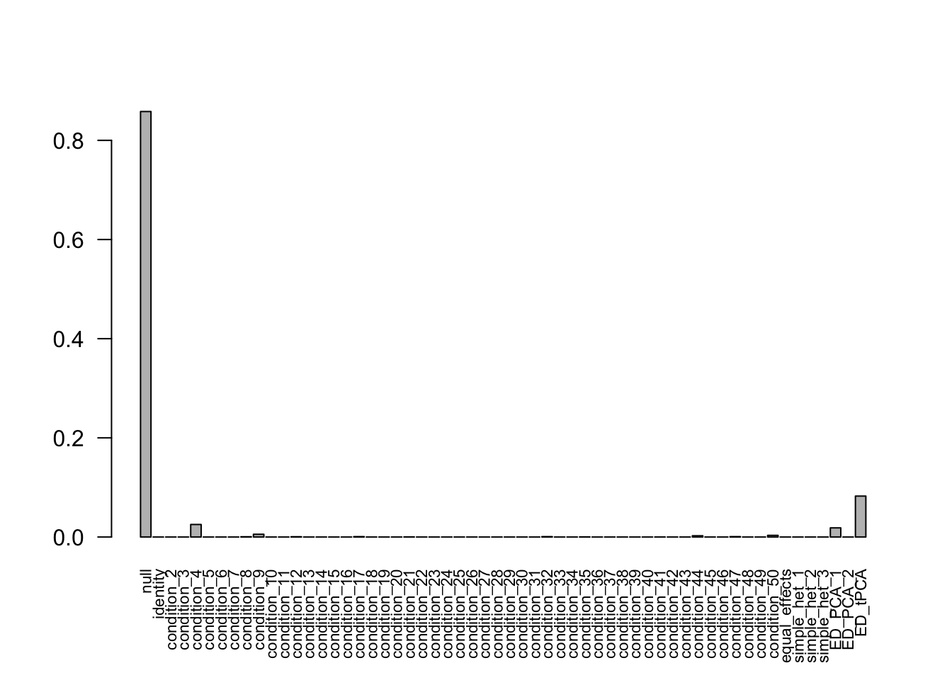
Recover the first column
mashcontrast.model.1.full = mashcontrast.model.1
mashcontrast.model.1.full$result = mash_compute_posterior_matrices(g = mashcontrast.model.1, data = mash_data_L.1, algorithm.version = 'R', recover=TRUE)
There are 609 discoveries.
Subtract mean directly
Indep.data.1 = mash_set_data(Bhat = mash_data_L.1$Bhat,
                           Shat = matrix(sqrt(0.5-1/(R*2)), nrow(data$Chat), R-1))

Indep.model.1 = mash(Indep.data.1, c(U.c, U.ed), algorithm.version = 'R', verbose = FALSE)
Warning in REBayes::KWDual(A, rep(1, k), normalize(w), control = control): estimated mixing distribution has some negative values:
consider reducing rtolWarning in mixIP(matrix_lik = structure(c(0.00667820972445308,
0.0631737437819963, : Optimization step yields mixture weights that are
either too small, or negative; weights have been corrected and renormalized
after the optimization.For mashIndep model, there are 606 discoveries. The covariance structure found here is:
barplot(get_estimated_pi(Indep.model.1),las = 2, cex.names = 0.7)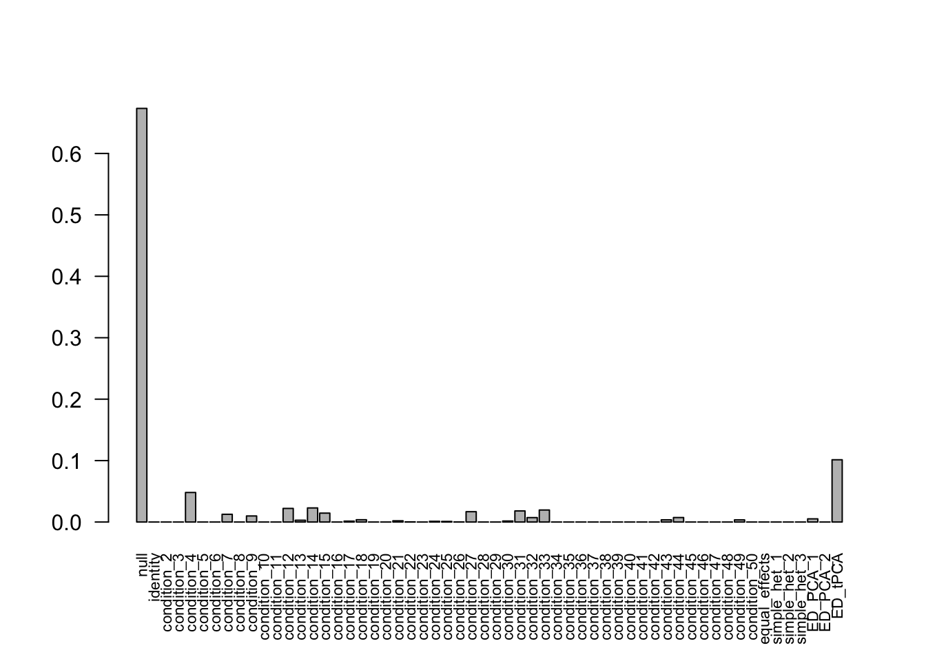
Recover the first column
Indep.model.1.full = Indep.model.1
Indep.model.1.full$result = mash_compute_posterior_matrices(g = Indep.model.1, data = Indep.data.1, algorithm.version = 'R', recover=TRUE)
There are 608 discoveries.
Compare models
The RRMSE plot:
delta.50 = data$C - rowMeans(data$C)
deltahat.50 = data$Chat - rowMeans(data$Chat)

delta.1 = delta.50[, c(2:50, 1)]
deltahat.1 = deltahat.50[, c(2:50, 1)]

barplot(c(sqrt(mean((delta.50 - mashcontrast.model.50.full$result$PosteriorMean)^2)/mean((delta.50 - deltahat.50)^2)), sqrt(mean((delta.1 - mashcontrast.model.1.full$result$PosteriorMean)^2)/mean((delta.1 - deltahat.1)^2)), sqrt(mean((delta.50 - Indep.model.50.full$result$PosteriorMean)^2)/mean((delta.50 - deltahat.50)^2)), sqrt(mean((delta.1 - Indep.model.1.full$result$PosteriorMean)^2)/mean((delta.1 - deltahat.1)^2))), ylim=c(0,0.2), names.arg = c('mashcommon.50','mashcommon.1','mash.indep.50', 'mash.indep.1'), ylab='RRMSE')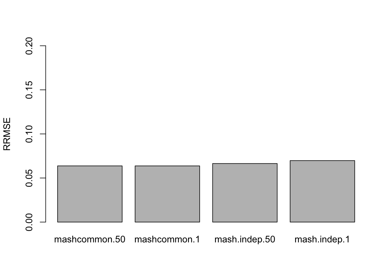
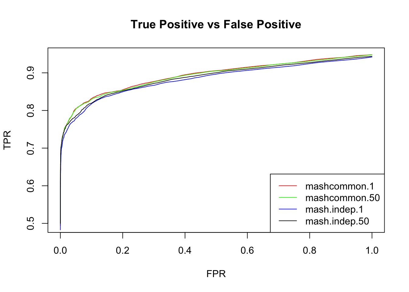
We check the False Positive Rate and True Positive Rate. \[FPR = \frac{|N\cap S|}{|N|} \quad TPR = \frac{|CS\cap S|}{|T|} \]
sign.test.mash.50 = as.matrix(delta.50)*mashcontrast.model.50.full$result$PosteriorMean
sign.test.Indep.50 = as.matrix(delta.50)*Indep.model.50.full$result$PosteriorMean
sign.test.mash.1 = as.matrix(delta.1)*mashcontrast.model.1.full$result$PosteriorMean
sign.test.Indep.1 = as.matrix(delta.1)*Indep.model.1.full$result$PosteriorMean

thresh.seq = seq(0, 1, by=0.0005)[-1]
mashcontrast.1 = matrix(0,length(thresh.seq), 2)
Indep.1 = matrix(0,length(thresh.seq), 2)
mashcontrast.50 = matrix(0,length(thresh.seq), 2)
Indep.50 = matrix(0,length(thresh.seq), 2)
colnames(mashcontrast.1) = c('TPR', 'FPR')
colnames(Indep.1) = c('TPR', 'FPR')
colnames(mashcontrast.50) = c('TPR', 'FPR')
colnames(Indep.50) = c('TPR', 'FPR')
for(t in 1:length(thresh.seq)){
  mashcontrast.1[t,] = c(sum(sign.test.mash.1>0 & mashcontrast.model.1.full$result$lfsr <= thresh.seq[t])/sum(delta.1!=0), sum(delta.1==0 & mashcontrast.model.1.full$result$lfsr <=thresh.seq[t])/sum(delta.1==0))

  Indep.1[t,] = c(sum(sign.test.Indep.1>0 & Indep.model.1.full$result$lfsr <= thresh.seq[t])/sum(delta.1!=0), sum(delta.1==0 & Indep.model.1.full$result$lfsr <=thresh.seq[t])/sum(delta.1==0))

  mashcontrast.50[t,] = c(sum(sign.test.mash.50>0 & mashcontrast.model.50.full$result$lfsr <= thresh.seq[t])/sum(delta.50!=0), sum(delta.50==0 & mashcontrast.model.50.full$result$lfsr <=thresh.seq[t])/sum(delta.50==0))

  Indep.50[t,] = c(sum(sign.test.Indep.50>0& Indep.model.50.full$result$lfsr <=thresh.seq[t])/sum(delta.50!=0), sum(delta.50==0& Indep.model.50.full$result$lfsr <=thresh.seq[t])/sum(delta.50==0))
}
Session information
sessionInfo()R version 3.4.4 (2018-03-15)
Platform: x86_64-apple-darwin15.6.0 (64-bit)
Running under: macOS High Sierra 10.13.4
Matrix products: default
BLAS: /Library/Frameworks/R.framework/Versions/3.4/Resources/lib/libRblas.0.dylib
LAPACK: /Library/Frameworks/R.framework/Versions/3.4/Resources/lib/libRlapack.dylib
locale:
[1] en_US.UTF-8/en_US.UTF-8/en_US.UTF-8/C/en_US.UTF-8/en_US.UTF-8
attached base packages:
[1] stats graphics grDevices utils datasets methods base
other attached packages:
[1] mvtnorm_1.0-7 plyr_1.8.4 assertthat_0.2.0 corrplot_0.84
[5] mashr_0.2-8 ashr_2.2-7
loaded via a namespace (and not attached):
[1] Rcpp_0.12.16 knitr_1.20
[3] magrittr_1.5 REBayes_1.3
[5] MASS_7.3-50 doParallel_1.0.11
[7] pscl_1.5.2 SQUAREM_2017.10-1
[9] lattice_0.20-35 ExtremeDeconvolution_1.3
[11] foreach_1.4.4 stringr_1.3.0
[13] tools_3.4.4 parallel_3.4.4
[15] grid_3.4.4 rmeta_3.0
[17] git2r_0.21.0 htmltools_0.3.6
[19] iterators_1.0.9 yaml_2.1.19
[21] rprojroot_1.3-2 digest_0.6.15
[23] Matrix_1.2-14 codetools_0.2-15
[25] evaluate_0.10.1 rmarkdown_1.9
[27] stringi_1.2.2 compiler_3.4.4
[29] Rmosek_8.0.69 backports_1.1.2
[31] truncnorm_1.0-8 This R Markdown site was created with workflowr