Table 2
Yuxin Zou
2018-2-1
Last updated: 2018-03-06
Code version: 866f1eb
library(gdata); library(mashr);library(flashr)gdata: read.xls support for 'XLS' (Excel 97-2004) files ENABLED.gdata: read.xls support for 'XLSX' (Excel 2007+) files ENABLED.
Attaching package: 'gdata'The following object is masked from 'package:stats':
nobsThe following object is masked from 'package:utils':
object.sizeThe following object is masked from 'package:base':
startsWithLoading required package: ashrlibrary(mclust); library(plyr); library(corrplot)Package 'mclust' version 5.4
Type 'citation("mclust")' for citing this R package in publications.
Attaching package: 'mclust'The following object is masked from 'package:ashr':
denscorrplot 0.84 loadedlibrary(ggplot2); library(ggpubr)Loading required package: magrittrRead Table 2
SupplTable2 = read.xls('../data/Suppl.Table.2.xlsx')
saveRDS(SupplTable2, '../data/SupplTable2.rds')
There are missing value in the data. I guess this is caused by the 0 count, since the effect is \(\log_{2} (X_{1}/X_{2})\). We set these NAs to 0 with huge variance.
Genename = as.character(SupplTable2$Gene.ID)
colname = colnames(SupplTable2)[seq(3,89,by=3)]
Tissue = gsub( "_.*$", "",  colname)

p.value = SupplTable2[,seq(3,89,by=3)]
logFC = SupplTable2[,seq(4,89,by=3)]

missing = is.na(as.matrix(logFC))

p.value[is.na(as.matrix(p.value))] = 1
logFC[is.na(as.matrix(logFC))] = 0

row.names(p.value) = Genename
row.names(logFC) = Genename
colnames(p.value) = Tissue
colnames(logFC) = Tissue

saveRDS(list(logFC = as.matrix(logFC), pval = as.matrix(p.value), category = SupplTable2$category, region = SupplTable2$region, missing = missing), '../data/SupplTable2_0.rds')
Since the sample size is large, we assume the p value is from normal distribution.
mash.data = mash_set_data(Bhat = data$logFC, pval = data$pval)
# set large variance to missing data
mash.data$Shat[is.na(mash.data$Shat)] = 1000
mash.data$Shat[is.infinite(mash.data$Shat)] = 1000

# find strong genes
m.1by1 = mash_1by1(mash.data, alpha=0)
strong = get_significant_results(m.1by1, 0.01)
# estimate cor V on non strong genes
Z = mash.data$Bhat/mash.data$Shat
Z.null = Z[setdiff(1:349,strong),]
Estimate covariance structure using strong genes
Z.strong = Z[strong,]
# center
Z.center = apply(Z.strong, 2, function(x) x - mean(x))
Flash
\[ \tilde{Z} = LF' + E \] where F is \(29 \times K\), L is \(n \times K\), E is \(n\times 29\).
mash_data_flash = flash_set_data(as.matrix(Z.center))
fmodel = flash(mash_data_flash, greedy = TRUE, backfit = TRUE)

saveRDS(fmodel, '../output/Flash_T2_0.rds')
Flash result
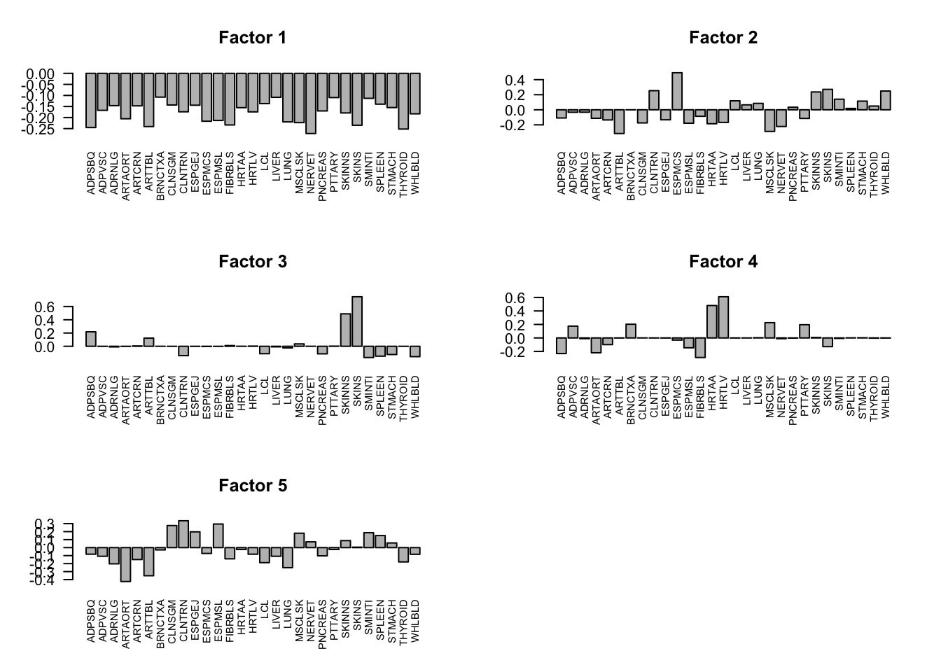
The first factor explains the main proportion of variance in effects.
flash_get_pve(fmodel)[1] 0.786204732 0.009596396 0.011735441 0.008650019 0.003879352The first factor is the overall summary of treatment effects.
factors = flash_get_ldf(fmodel)$f
row.names(factors) = colnames(data$logFC)
layout(matrix(c(1,2,3,4,5,6), 3, 2, byrow = TRUE))
for(i in 1:5){
  barplot(factors[,i], las=2, main=paste0('Factor ', i), cex.names = 0.7)
}
Clustering loadings
loading = fmodel$EL[,1:5]
row.names(loading) = rownames(Z.strong)
colnames(loading) = paste0('F',seq(1,5))

mod = Mclust(loading)
summary(mod$BIC)
saveRDS(mod, '../output/Flash_T2_0_mclust.rds')
Using clustering result to fit mash:
\[l_{i}\sim \sum_{i=1}^{m}N(\mu_{i}, \Sigma_{i})\] We estimate the covariance as \(F(\Sigma_i + \mu_{i}\mu_{i}')F'\).
U_list = alply(mod$parameters$variance$sigma,3)
mu_list = alply(mod$parameters$mean,2)
ll = list()
for (i in 1:length(U_list)){
  ll[[i]] = U_list[[i]] + mu_list[[i]] %*% t(mu_list[[i]])
}

U.loading = lapply(ll, function(U){factors %*% (U %*% t(factors))})
names(U.loading) = paste0('Load', "_", (1:length(U.loading)))

# rank 1

Flash_res = flash_get_lf(fmodel)

U.Flash = c(mashr::cov_from_factors(t(as.matrix(factors)), "Flash"),
            list("tFlash" = t(Flash_res) %*% Flash_res / nrow(Z.center)))
PCA
U.pca = cov_pca(mash_set_data(Z.center), 7)Canonical
U.c = cov_canonical(mash_set_data(Z.center))Extreme Deconvolution
U.dd = c(U.pca, U.loading, U.Flash, list('XX' = t(Z.center) %*% Z.center / nrow(Z.center) ))

mash.data.ed = mash.data
mash.data.ed$Bhat = mash.data$Bhat[strong,]
mash.data.ed$Shat = mash.data$Shat[strong,]
mash.data.ed$Shat_alpha = mash.data$Shat_alpha[strong,]
saveRDS(cov_ed(mash.data.ed, U.dd), '../output/Mash_EE_Cov_0_plusR1.rds')
mash model
vhat = 1

if (vhat == 1) {
  V = cor(Z.null)
} else {
  V = diag(ncol(Z.null))
}

mash_data = mash_set_data(Bhat = mash.data$Bhat, Shat = mash.data$Shat, V = V, alpha = 0)

saveRDS(mash(mash_data, c(U.c, U.ed)), '../output/Mash_model_0_plusR1.rds')
- Computing 959 x 1711 likelihood matrix.
- Likelihood calculations took 17.60 seconds.
- Fitting model with 1711 mixture components.
- Model fitting took 15.55 seconds.
- Computing posterior matrices.
- Computation allocated took 3.72 seconds.V1 EE result
The log-likelihood of fit is
get_loglik(mash.model)[1] -80852.06Here is a plot of weights learned.
options(repr.plot.width=12, repr.plot.height=4)
barplot(get_estimated_pi(mash.model), las = 2, cex.names = 0.7)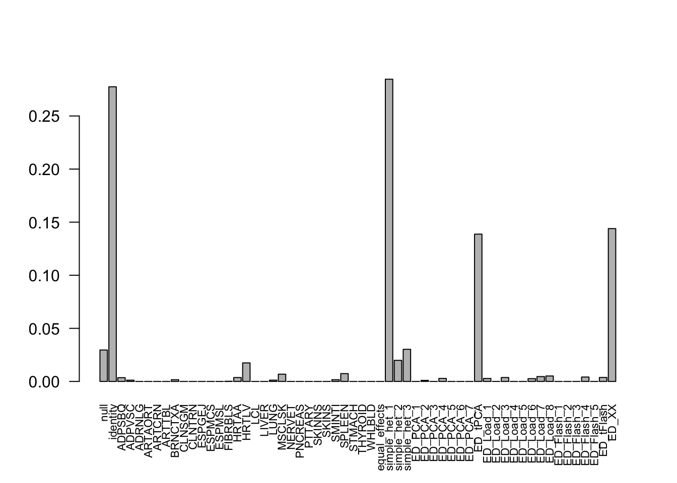
Check ED_XX and ED_tPCA:
layout(matrix(c(1,2,3,4), 2, 2, byrow=TRUE))
svd.out = svd(mash.model$fitted_g$Ulist[["ED_XX"]])
v = svd.out$v
colnames(v) = colnames(get_lfsr(mash.model))
rownames(v) = colnames(v)
options(repr.plot.width=10, repr.plot.height=5)
for (j in 1:4)
  barplot(v[,j]/v[,j][which.max(abs(v[,j]))], cex.names = 0.7,
          las = 2, main = paste0("EigenVector ", j, " for XX"))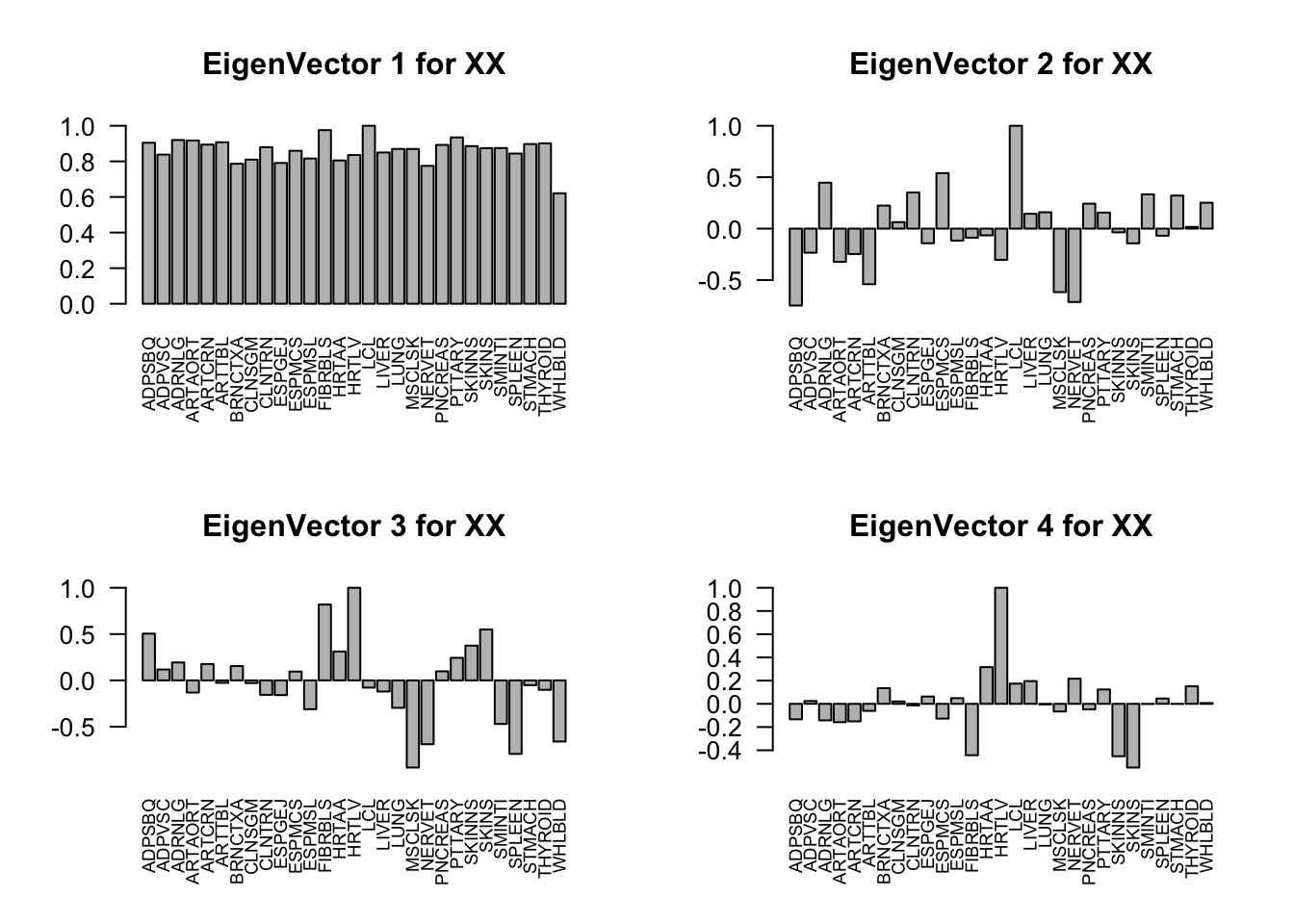
svd.out = svd(mash.model$fitted_g$Ulist[["ED_tPCA"]])
v = svd.out$v
colnames(v) = colnames(get_lfsr(mash.model))
rownames(v) = colnames(v)
options(repr.plot.width=10, repr.plot.height=5)
for (j in 1:4)
  barplot(v[,j]/v[,j][which.max(abs(v[,j]))], cex.names = 0.7,
          las = 2, main = paste0("EigenVector ", j, " for tPCA"))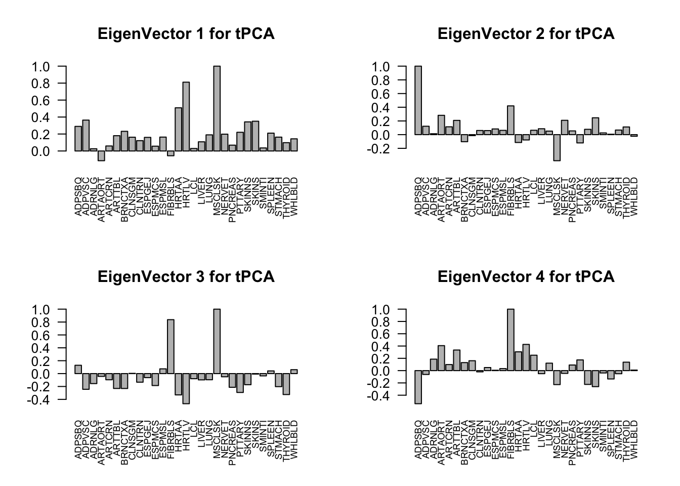
Among the 959 genes, MASH found 372 to be significant in at least one treatment.
There are 84 effects are estimated as significant, even though they are originally missing! This is caused by the borrowing information from other samples.
The plot below compares the data with the mash output. The gene ASMT has lots of missing vales in tissues. The mash model estimates all effects as significant.
# before
gene667 = data.frame(mash.data$Bhat[667,])
colnames(gene667) = 'EffectSize'
gene667$Group = row.names(gene667)
gene667$se = data.frame(ifelse(mash.data$Shat[667,]>100, 0, mash.data$Shat[667,]))
gene667$EffectSize[gene667$se == 0] = NA
# after
gene667.post = data.frame(mash.model$result$PosteriorMean[667,])
colnames(gene667.post) = 'EffectSize'
gene667.post$Group = row.names(gene667)
gene667.post$se = data.frame(mash.model$result$PosteriorSD[667,])

p.orig = ggplot(gene667, aes(y = EffectSize, x = Group, color=Group)) +
  geom_point() +
  geom_errorbar(aes(ymin=EffectSize-1.96*se, ymax=EffectSize+1.96*se), width=0.4) +
  theme_bw(base_size=12) + coord_flip() + ggtitle('ASMT original' )

p.post = ggplot(gene667.post, aes(y = EffectSize, x = Group, color=Group)) +
  geom_point() +
  geom_errorbar(aes(ymin=EffectSize-1.96*se, ymax=EffectSize+1.96*se), width=0.4) +
  theme_bw(base_size=12) + coord_flip() + ggtitle('ASMT mash') + theme(legend.position = 'bottom')

ggarrange(p.orig, p.post, ncol=2, nrow=1, common.legend = TRUE, legend="right")
Warning: Removed 24 rows containing missing values (geom_point).Warning: Removed 24 rows containing missing values (geom_errorbar).Warning: Removed 24 rows containing missing values (geom_point).Warning: Removed 24 rows containing missing values (geom_errorbar).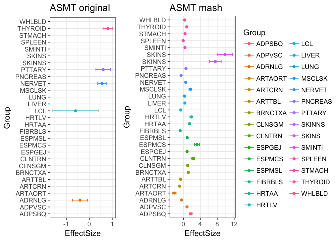
Proportion of significantly biased (FDR < 1%) genes in each tissue by reported XCI status.
Escape.prop = numeric(29)
for(i in 1:29){
  Escape.prop[i] = length(which(data$category[get_significant_results(mash.model,0.01, conditions = i)] == 'Escape')) / length(which(data$category == 'Escape'))
}
Variable.prop = numeric(29)
for(i in 1:29){
  Variable.prop[i] = length(which(data$category[get_significant_results(mash.model,0.01, conditions = i)] == 'Variable')) / length(which(data$category == 'Variable'))
}
Inac.prop = numeric(29)
for(i in 1:29){
  Inac.prop[i] = length(which(data$category[get_significant_results(mash.model,0.01, conditions = i)] == 'Inactive')) / length(which(data$category == 'Inactive'))
}
Unknown.prop = numeric(29)
for(i in 1:29){
  Unknown.prop[i] = length(which(data$category[get_significant_results(mash.model,0.01, conditions = i)] == 'Unknown')) / length(which(data$category == 'Unknown'))
}

prop = c(Escape.prop, Variable.prop, Inac.prop, Unknown.prop)
group = rep(c('Escape', 'Variable', 'Inactive', 'Unknown'), each=29)
boxplot(prop*100~group, ylab='Sex-bias per tissue (% of genes)')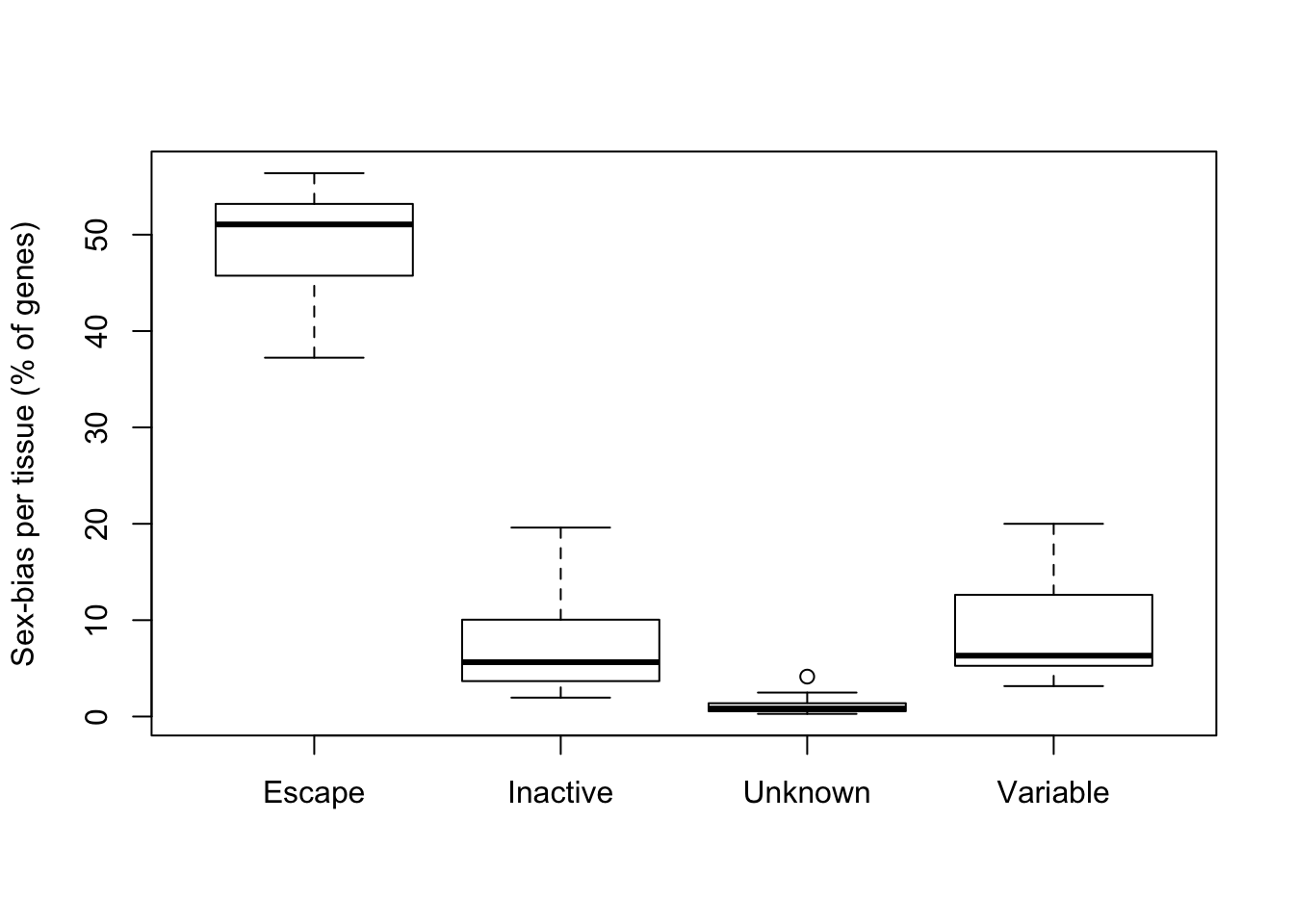
Sex biased expression is enriched in escape genes.
Session information
sessionInfo()R version 3.4.3 (2017-11-30)
Platform: x86_64-apple-darwin15.6.0 (64-bit)
Running under: macOS High Sierra 10.13.3
Matrix products: default
BLAS: /Library/Frameworks/R.framework/Versions/3.4/Resources/lib/libRblas.0.dylib
LAPACK: /Library/Frameworks/R.framework/Versions/3.4/Resources/lib/libRlapack.dylib
locale:
[1] en_US.UTF-8/en_US.UTF-8/en_US.UTF-8/C/en_US.UTF-8/en_US.UTF-8
attached base packages:
[1] stats graphics grDevices utils datasets methods base
other attached packages:
[1] ggpubr_0.1.6 magrittr_1.5 ggplot2_2.2.1 corrplot_0.84 plyr_1.8.4
[6] mclust_5.4 flashr_0.5-6 mashr_0.2-6 ashr_2.2-7 gdata_2.18.0
loaded via a namespace (and not attached):
[1] Rcpp_0.12.15 bindr_0.1 compiler_3.4.3
[4] git2r_0.20.0 iterators_1.0.9 tools_3.4.3
[7] digest_0.6.13 tibble_1.3.4 evaluate_0.10.1
[10] gtable_0.2.0 lattice_0.20-35 pkgconfig_2.0.1
[13] rlang_0.1.6 Matrix_1.2-12 foreach_1.4.4
[16] yaml_2.1.17 parallel_3.4.3 mvtnorm_1.0-7
[19] ebnm_0.1-10 bindrcpp_0.2 gridExtra_2.3
[22] dplyr_0.7.4 stringr_1.3.0 knitr_1.20
[25] REBayes_1.2 gtools_3.5.0 cowplot_0.9.2
[28] rprojroot_1.2 grid_3.4.3 glue_1.2.0
[31] R6_2.2.2 rmarkdown_1.8 rmeta_2.16
[34] purrr_0.2.4 backports_1.1.2 scales_0.5.0
[37] codetools_0.2-15 htmltools_0.3.6 MASS_7.3-47
[40] assertthat_0.2.0 softImpute_1.4 colorspace_1.3-2
[43] labeling_0.3 stringi_1.1.6 Rmosek_8.0.69
[46] lazyeval_0.2.1 doParallel_1.0.11 pscl_1.5.2
[49] munsell_0.4.3 truncnorm_1.0-8 SQUAREM_2017.10-1This R Markdown site was created with workflowr