Mashcommonbaseline

Last updated: 2018-05-12

workflowr checks: (Click a bullet for more information)

✔ R Markdown file: up-to-date

Great! Since the R Markdown file has been committed to the Git repository, you know the exact version of the code that produced these results.
✔ Environment: empty

Great job! The global environment was empty. Objects defined in the global environment can affect the analysis in your R Markdown file in unknown ways. For reproduciblity it’s best to always run the code in an empty environment.
✔ Seed: set.seed(20180510)

The command set.seed(20180510) was run prior to running the code in the R Markdown file. Setting a seed ensures that any results that rely on randomness, e.g. subsampling or permutations, are reproducible.
✔ Session information: recorded

Great job! Recording the operating system, R version, and package versions is critical for reproducibility.
✔ Repository version: 326232c
Great! You are using Git for version control. Tracking code development and connecting the code version to the results is critical for reproducibility. The version displayed above was the version of the Git repository at the time these results were generated.

Note that you need to be careful to ensure that all relevant files for the analysis have been committed to Git prior to generating the results (you can use wflow_publish or wflow_git_commit). workflowr only checks the R Markdown file, but you know if there are other scripts or data files that it depends on. Below is the status of the Git repository when the results were generated:
```
Ignored files:
    Ignored:    .Rhistory
    Ignored:    .Rproj.user/

Untracked files:
    Untracked:  .DS_Store
    Untracked:  data/.DS_Store
    Untracked:  data/raw_data/
    Untracked:  data/results/.DS_Store
    Untracked:  data/results/tables/
    Untracked:  data/working_data/
```
Note that any generated files, e.g. HTML, png, CSS, etc., are not included in this status report because it is ok for generated content to have uncommitted changes.

Expand here to see past versions:

File	Version	Author	Date	Message
Rmd	326232c	zouyuxin	2018-05-12	wflow_publish(“analysis/MashCommonbaseline.Rmd”)
html	4a8a857	zouyuxin	2018-05-12	Build site.
Rmd	12acda1	zouyuxin	2018-05-12	wflow_publish(“analysis/MashCommonbaseline.Rmd”)
html	c74944f	zouyuxin	2018-05-11	Build site.
Rmd	24354db	zouyuxin	2018-05-11	mash models
html	5148e0b	zouyuxin	2018-05-10	Build site.
Rmd	9dae4f1	zouyuxin	2018-05-10	wflow_publish(“analysis/MashCommonbaseline.Rmd”)
html	60c0e2f	zouyuxin	2018-05-10	Build site.
Rmd	fc22b3f	zouyuxin	2018-05-10	wflow_publish(“analysis/MashCommonbaseline.Rmd”)

library(limma); library(mashr); library(mclust); library(plyr);

Loading required package: ashr

Package 'mclust' version 5.4
Type 'citation("mclust")' for citing this R package in publications.


Attaching package: 'mclust'

The following object is masked from 'package:ashr':

    dens

library(flashr); library(colorRamps); library(corrplot)

corrplot 0.84 loaded

data = readRDS('../data/results/Microarray_compiledGLM.rds')

Mash

The standard errors in the data are from t distribution with df 452. Since pt(-abs(Bhat/Shat), df) is very close to zero, it is hard to obtain the standard error from the normal distribution. The degree of freedom is large here, we use the original standard error.

mash.data = mash_set_data(Bhat = data$Chat, Shat = data$SE)
L = diag(ncol(data$Chat))
# the 4th col is CTL
L[,4] = -1
row.names(L) = colnames(data$Chat)
L = L[-4,]
mash.data.diff = mash_set_data_contrast(mash.data, L)

Top genes:

# find strong genes
m.1by1 = mash_1by1(mash.data.diff, alpha=0)
strong = get_significant_results(m.1by1)
# almost all genes are strong
set.seed(100)
strong.sample = sample(strong, length(strong)/2, replace = FALSE)
Z = mash.data.diff$Bhat/mash.data.diff$Shat
Z.strong = Z[strong.sample,]
# center
Z.center = apply(Z.strong, 2, function(x) x - mean(x))

Estimate covariance structures:

Data Driven:

Flash:

flash.data = flash_set_data(Z.center)
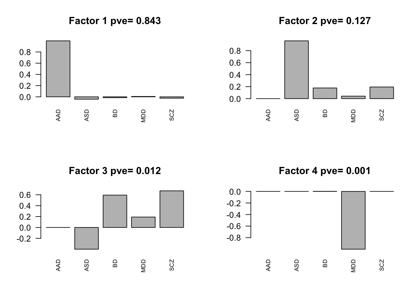
fmodel = flash(flash.data, greedy = TRUE, backfit = TRUE)

fitting factor/loading 1

fitting factor/loading 2

fitting factor/loading 3

fitting factor/loading 4

fitting factor/loading 5

factors = flash_get_ldf(fmodel)$f
row.names(factors) = row.names(L)
pve.order = order(flash_get_pve(fmodel), decreasing = TRUE)

par(mfrow=c(2,2))
for(i in pve.order){
  barplot(factors[,i], main=paste0('Factor ',i, ' pve= ', round(flash_get_pve(fmodel)[i],3)), las=2, cex.names = 0.7)
}

Expand here to see past versions of flash plot-1.png:

Version	Author	Date
4a8a857	zouyuxin	2018-05-12
5148e0b	zouyuxin	2018-05-10
60c0e2f	zouyuxin	2018-05-10

par(mfrow=c(1,1))

flash on the loading:

loading = fmodel$EL[,1:4]
colnames(loading) = paste0('Factor',seq(1,4))
flash.loading = flash_set_data(loading)
flmodel = flash(flash.loading, greedy = TRUE, backfit = TRUE)

fitting factor/loading 1

The flash prefers the rank 0 model. There is no hidden structure in the loading matrix.

Cluster loadings:

mod = Mclust(loading)
summary(mod$BIC)

Best BIC values:
            VVI,9      VVE,9     VVE,8
BIC      3861.542 3822.14394 3744.2387
BIC diff    0.000  -39.39761 -117.3028

Using clustering result to fit mash:

\[l_{i}\sim \sum_{j=1}^{m}N(\mu_{j}, \Sigma_{j})\] We estimate the covariance as \(F(\Sigma_j + \mu_{j}\mu_{j}')F'\).

U_list = alply(mod$parameters$variance$sigma,3)
mu_list = alply(mod$parameters$mean,2)
ll = list()
for (i in 1:length(U_list)){
  ll[[i]] = U_list[[i]] + mu_list[[i]] %*% t(mu_list[[i]])
}

Factors = fmodel$EF[,1:4]
U.loading = lapply(ll, function(U){Factors %*% (U %*% t(Factors))})
names(U.loading) = paste0('Load', "_", (1:length(U.loading)))

# rank 1
Flash_res = flash_get_lf(fmodel)
U.Flash = c(mashr::cov_from_factors(t(as.matrix(factors)), "Flash"), 
            list("tFlash" = t(Flash_res) %*% Flash_res / nrow(Z.center)))

PCA:

U.pca = cov_pca(mash_set_data(Z.center), 3)

Canonical

U.c = cov_canonical(mash_set_data(Z.center))

Extreme Deconvolution

U.dd = c(U.pca, U.loading, U.Flash, list('XX' = t(Z.center) %*% Z.center / nrow(Z.center)))

mash.data.ed = mash.data.diff
mash.data.ed$Bhat = mash.data.diff$Bhat[strong,]
mash.data.ed$Shat = mash.data.diff$Shat[strong,]
mash.data.ed$Shat_alpha = mash.data.diff$Shat_alpha[strong,]
saveRDS(cov_ed(mash.data.ed, U.dd), '../output/MashCB_EE_Cov.rds')

Mash model:

U.ed = readRDS('../output/MashCB_EE_Cov.rds')

saveRDS(mash(mash.data.diff, c(U.c, U.ed), algorithm.version = 'R'), '../output/MashCB_model_EE.rds')

Result

mash.model = readRDS('../output/MashCB_model_EE.rds')

The log-likelihood of fit is

get_loglik(mash.model)

[1] 65270.31

Here is a plot of weights learned:

options(repr.plot.width=12, repr.plot.height=4)
barplot(get_estimated_pi(mash.model), las = 2, cex.names = 0.7)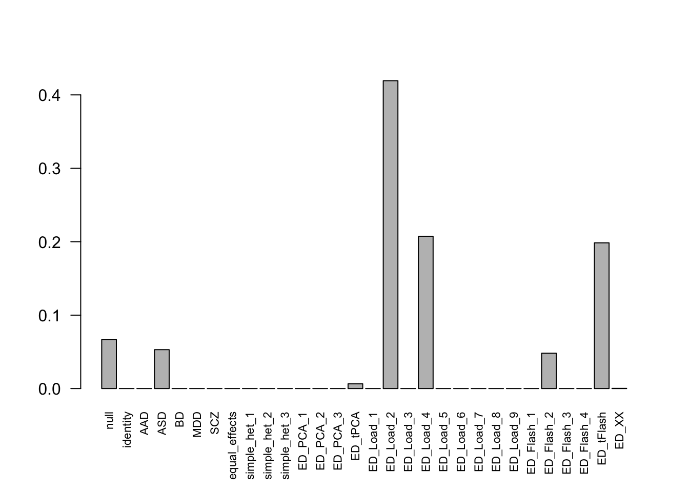

Expand here to see past versions of estimated weight-1.png:

Version	Author	Date
4a8a857	zouyuxin	2018-05-12
5148e0b	zouyuxin	2018-05-10
60c0e2f	zouyuxin	2018-05-10

Check Load 2 covariance matrix

x           <- mash.model$fitted_g$Ulist[["ED_Load_2"]]
colnames(x) <- row.names(L)
rownames(x) <- colnames(x)
corrplot(x, method='color', cl.lim=c(-0.2,1), type='upper', addCoef.col = "black", tl.col="black", tl.srt=45, col=colorRampPalette(c("blue","white","red"))(200))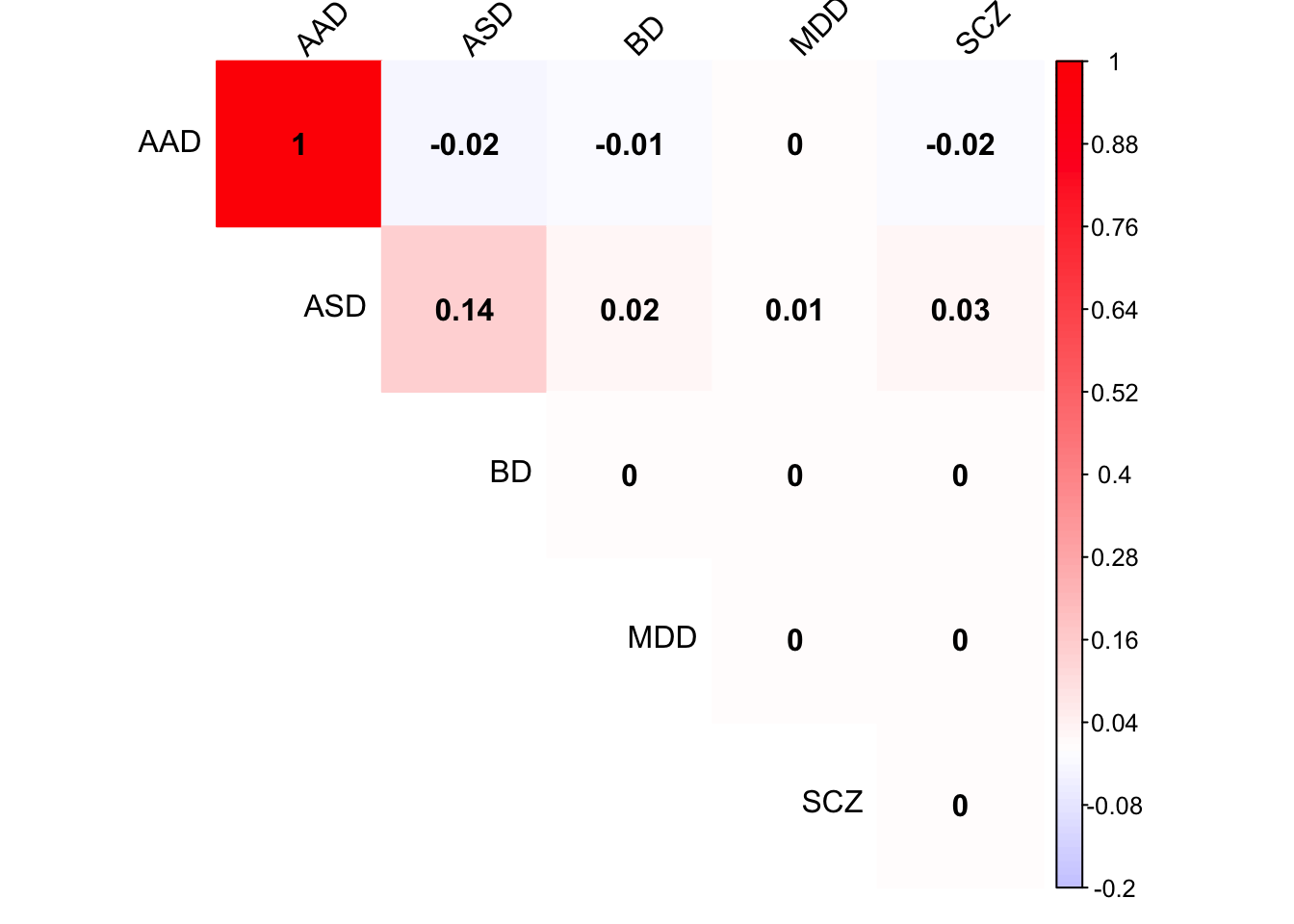

Expand here to see past versions of Load2-1.png:

Version	Author	Date
4a8a857	zouyuxin	2018-05-12

layout(matrix(c(1,2,3,4), 2, 2, byrow=TRUE))
svd.out = svd(mash.model$fitted_g$Ulist[["ED_Load_2"]])
v = svd.out$v
colnames(v) = row.names(L)
rownames(v) = colnames(v)
options(repr.plot.width=10, repr.plot.height=5)
for (j in 1:4)
  barplot(v[,j]/v[,j][which.max(abs(v[,j]))], cex.names = 0.7,
          las = 2, main = paste0("EigenVector ", j, " for Load 2"))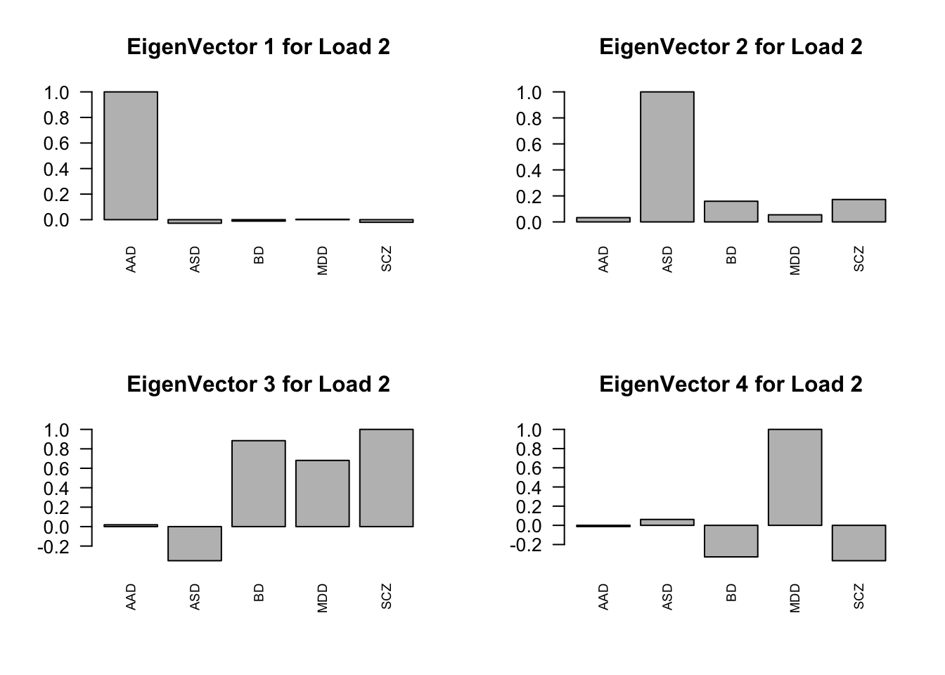

Expand here to see past versions of Load2 pca-1.png:

Version	Author	Date
4a8a857	zouyuxin	2018-05-12

Check Load 4 covariance matrix

x           <- mash.model$fitted_g$Ulist[["ED_Load_4"]]
colnames(x) <- row.names(L)
rownames(x) <- colnames(x)
corrplot(x, method='color', cl.lim=c(-0.2,1), type='upper', addCoef.col = "black", tl.col="black", tl.srt=45, col=colorRampPalette(c("blue","white","red"))(200))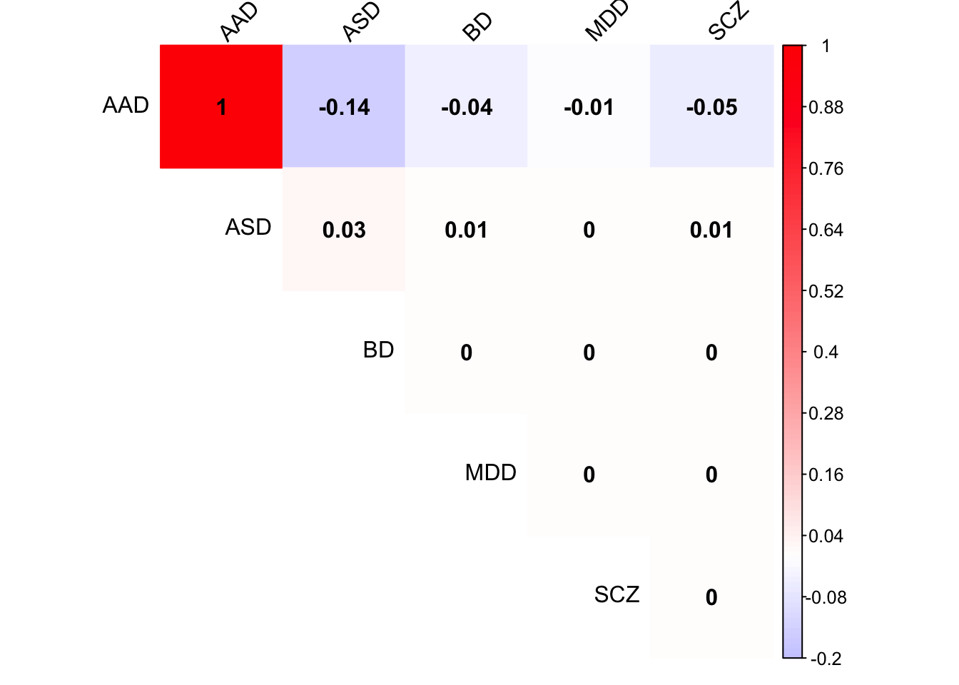

Expand here to see past versions of Load4-1.png:

Version	Author	Date
4a8a857	zouyuxin	2018-05-12
5148e0b	zouyuxin	2018-05-10

layout(matrix(c(1,2,3,4), 2, 2, byrow=TRUE))
svd.out = svd(mash.model$fitted_g$Ulist[["ED_Load_4"]])
v = svd.out$v
colnames(v) = row.names(L)
rownames(v) = colnames(v)
options(repr.plot.width=10, repr.plot.height=5)
for (j in 1:4)
  barplot(v[,j]/v[,j][which.max(abs(v[,j]))], cex.names = 0.7,
          las = 2, main = paste0("EigenVector ", j, " for Load 4"))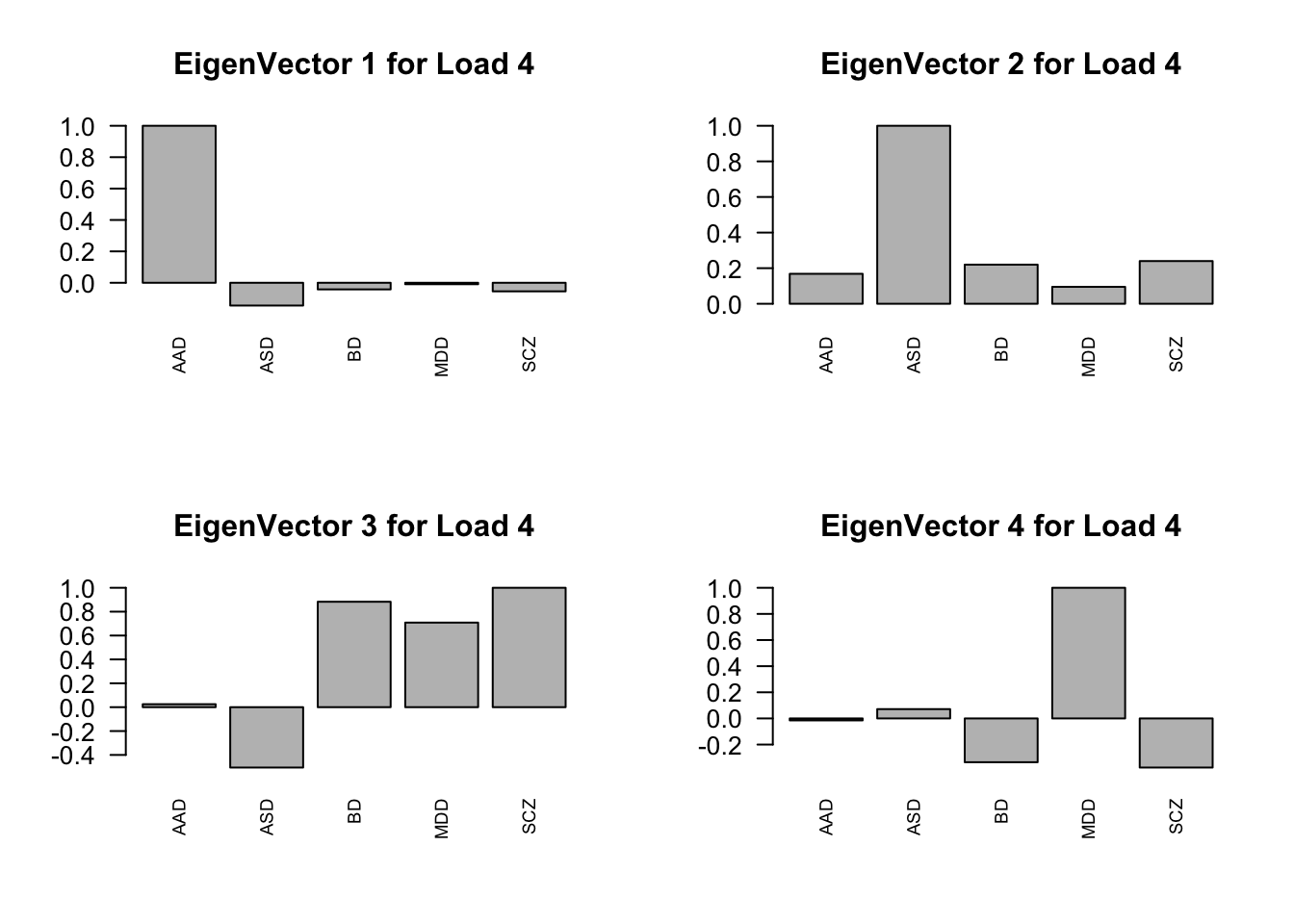

Expand here to see past versions of Load4 pca-1.png:

Version	Author	Date
4a8a857	zouyuxin	2018-05-12
5148e0b	zouyuxin	2018-05-10

Check tFlash covariance matrix

x           <- mash.model$fitted_g$Ulist[["ED_tFlash"]]
colnames(x) <- row.names(L)
rownames(x) <- colnames(x)
corrplot(x, method='color', cl.lim=c(-0.1,1), type='upper', addCoef.col = "black", tl.col="black", tl.srt=45, col=colorRampPalette(c("blue","white","red"))(200))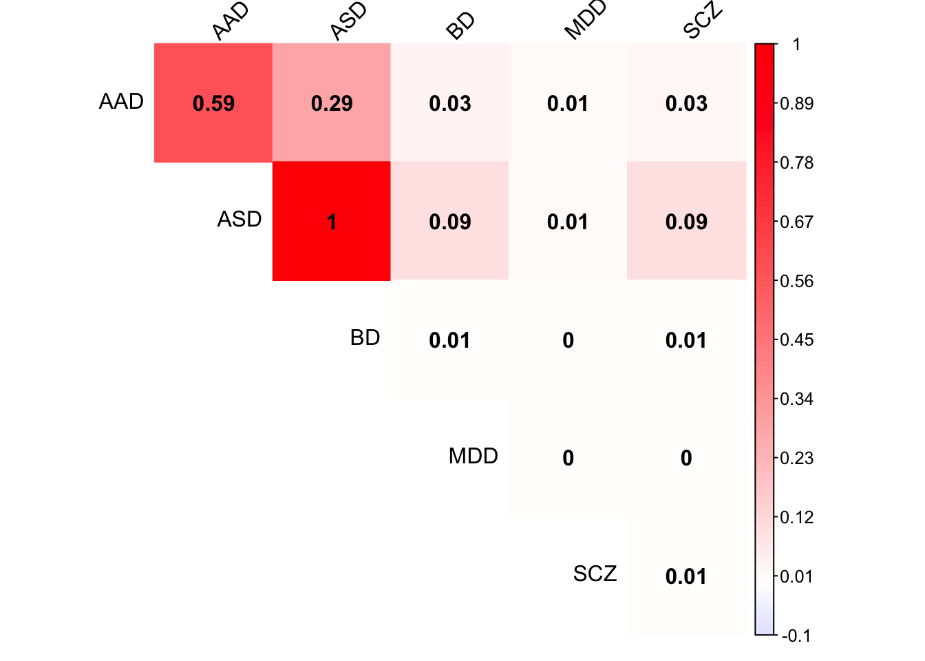

Expand here to see past versions of tFlash-1.png:

Version	Author	Date
4a8a857	zouyuxin	2018-05-12

layout(matrix(c(1,2,3,4), 2, 2, byrow=TRUE))
svd.out = svd(mash.model$fitted_g$Ulist[["ED_tFlash"]])
v = svd.out$v
colnames(v) = row.names(L)
rownames(v) = colnames(v)
options(repr.plot.width=10, repr.plot.height=5)
for (j in 1:4)
  barplot(v[,j]/v[,j][which.max(abs(v[,j]))], cex.names = 0.7,
          las = 2, main = paste0("EigenVector ", j, " for tFlash"))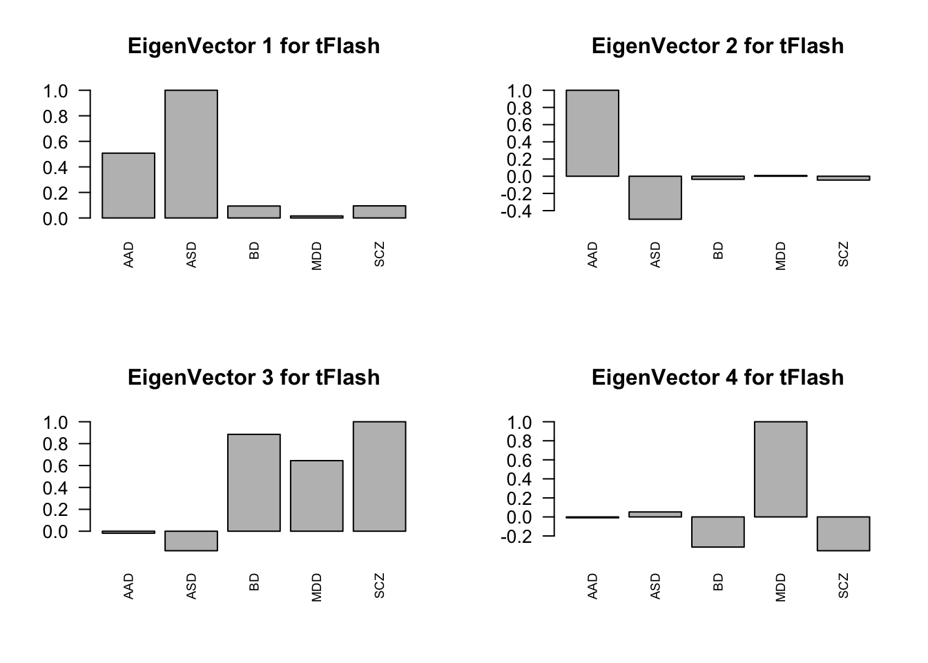

Expand here to see past versions of tFlash pca-1.png:

Version	Author	Date
4a8a857	zouyuxin	2018-05-12

Check Flash2 covariance matrix

x           <- mash.model$fitted_g$Ulist[["ED_Flash_2"]]
colnames(x) <- row.names(L)
rownames(x) <- colnames(x)
corrplot(x, method='color', cl.lim=c(-0.1,1), type='upper', addCoef.col = "black", tl.col="black", tl.srt=45, col=colorRampPalette(c("blue","white","red"))(200))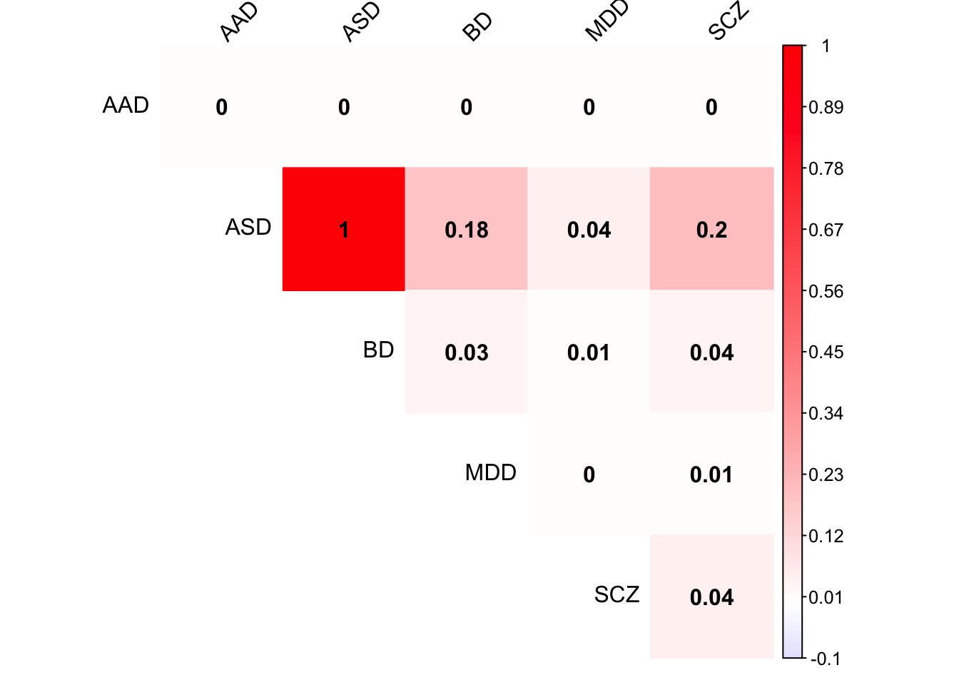

Expand here to see past versions of Flash2-1.png:

Version	Author	Date
4a8a857	zouyuxin	2018-05-12

layout(matrix(c(1,2,3,4), 2, 2, byrow=TRUE))
svd.out = svd(mash.model$fitted_g$Ulist[["ED_Flash_2"]])
v = svd.out$v
colnames(v) = row.names(L)
rownames(v) = colnames(v)
options(repr.plot.width=10, repr.plot.height=5)
for (j in 1:4)
  barplot(v[,j]/v[,j][which.max(abs(v[,j]))], cex.names = 0.7,
          las = 2, main = paste0("EigenVector ", j, " for Flash 2"))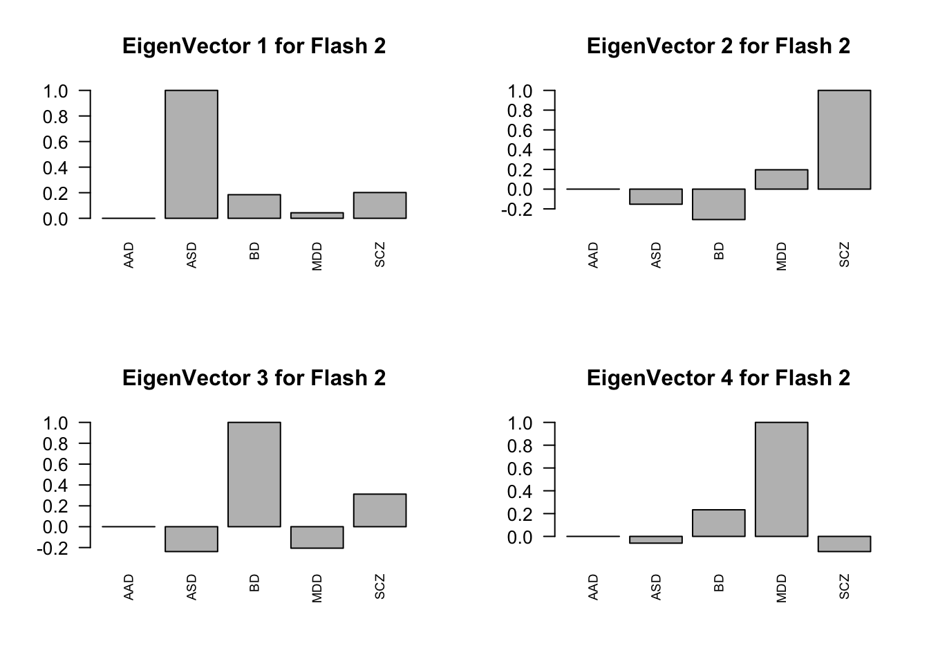

Expand here to see past versions of Flash2 pca-1.png:

Version	Author	Date
4a8a857	zouyuxin	2018-05-12

There are 4427 diferentially expressed genes.

Check pairwise sharing by sign:

x = get_pairwise_sharing(mash.model, factor=0)
x[x > 1]    <- 1
x[x < -1]   <- -1
colnames(x) <- row.names(L)
rownames(x) <- colnames(x)
corrplot.mixed(x, tl.pos="d",upper='color', cl.lim=c(0,1), upper.col=colorRampPalette(rev(c("#D73027","#FC8D59","#FEE090","#FFFFBF",
                               "#E0F3F8","#91BFDB","#4575B4")))(40),
               tl.cex=1.2)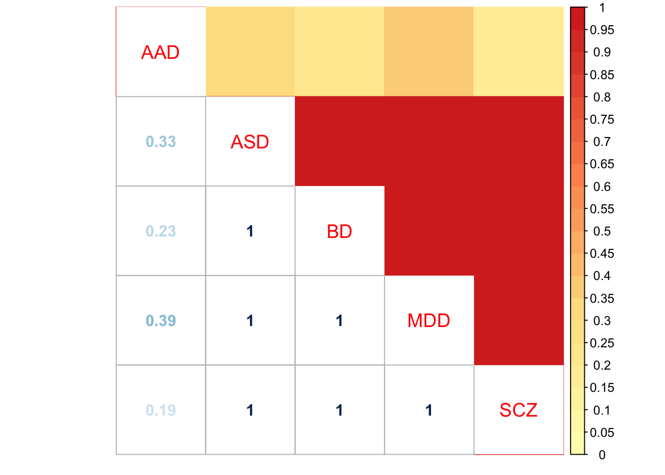

Expand here to see past versions of unnamed-chunk-3-1.png:

Version	Author	Date
4a8a857	zouyuxin	2018-05-12
5148e0b	zouyuxin	2018-05-10
60c0e2f	zouyuxin	2018-05-10

Check pairwise sharing by magnitude and sign:

x = get_pairwise_sharing(mash.model)
x[x > 1]    <- 1
x[x < -1]   <- -1
colnames(x) <- row.names(L)
rownames(x) <- colnames(x)
corrplot.mixed(x, tl.pos="d",upper='color', cl.lim=c(0,1), upper.col=colorRampPalette(rev(c("#D73027","#FC8D59","#FEE090","#FFFFBF",
                               "#E0F3F8","#91BFDB","#4575B4")))(40),
               tl.cex=1.2)

Expand here to see past versions of unnamed-chunk-4-1.png:

Version	Author	Date
4a8a857	zouyuxin	2018-05-12
5148e0b	zouyuxin	2018-05-10
60c0e2f	zouyuxin	2018-05-10

Effects compare with SCZ

CompareSCZ = diag(5)
CompareSCZ[,5] = -1
CompareSCZ = CompareSCZ[-5,]
row.names(CompareSCZ) = colnames(mash.data.diff$Bhat)[-5]

mash.model.SCZ = mash.model
mash.model.SCZ$result = mash_compute_posterior_matrices(mash.model, mash.data.diff, A=CompareSCZ, algorithm.version = 'R')
saveRDS(mash.model.SCZ, '../output/MashCB_model_EE_CompareSCZ.rds')

Check pairwise sharing by sign:

x = get_pairwise_sharing(mash.model.SCZ, factor=0)
x[x > 1]    <- 1
x[x < -1]   <- -1
colnames(x) <- row.names(CompareSCZ)
rownames(x) <- colnames(x)
corrplot.mixed(x, tl.pos="d",upper='color', cl.lim=c(0,1), upper.col=colorRampPalette(rev(c("#D73027","#FC8D59","#FEE090","#FFFFBF",
                               "#E0F3F8","#91BFDB","#4575B4")))(40),
               tl.cex=1.2)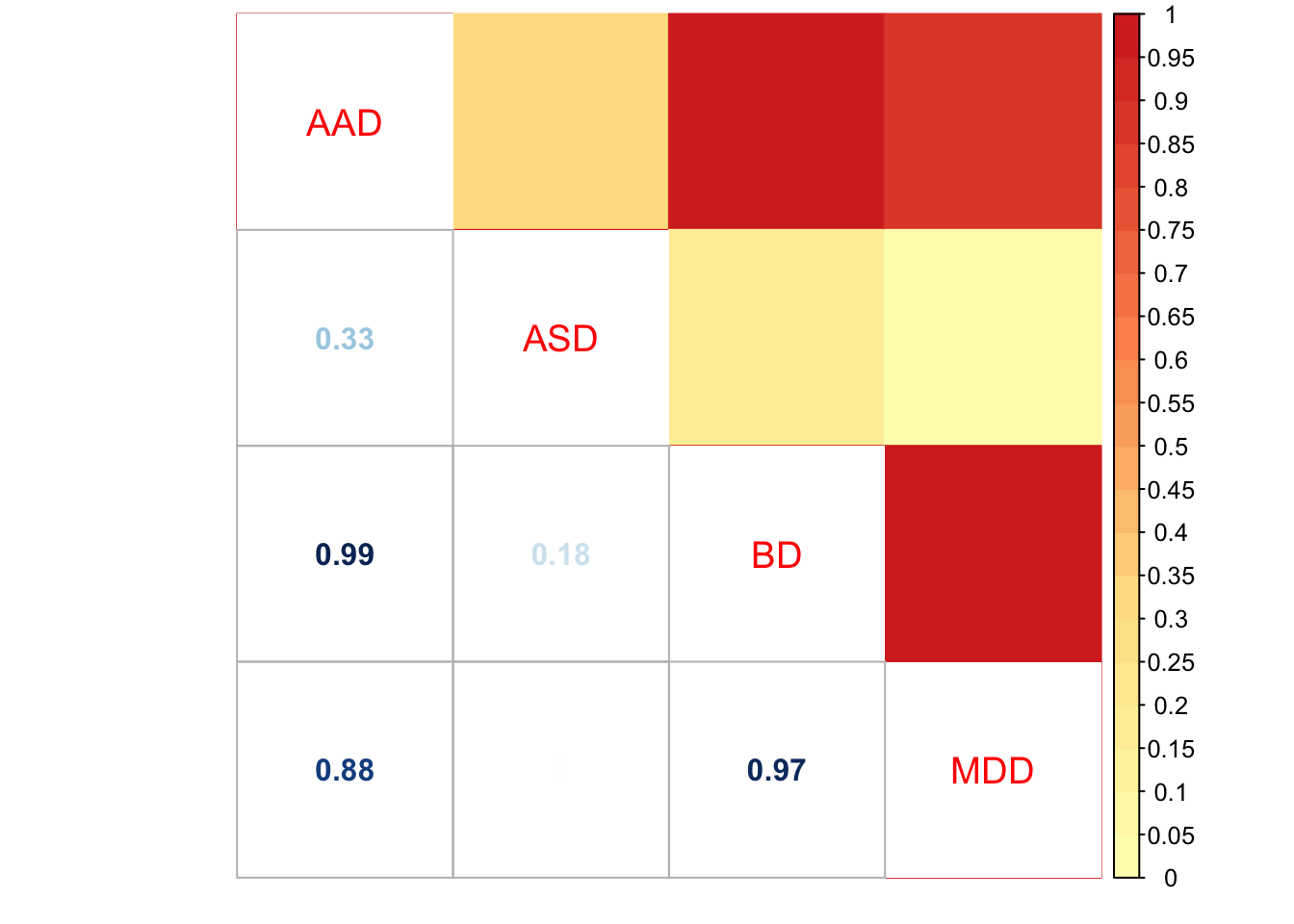

Expand here to see past versions of unnamed-chunk-8-1.png:

Version	Author	Date
4a8a857	zouyuxin	2018-05-12

Check pairwise sharing by magnitude and sign:

x = get_pairwise_sharing(mash.model.SCZ)
x[x > 1]    <- 1
x[x < -1]   <- -1
colnames(x) <- row.names(CompareSCZ)
rownames(x) <- colnames(x)
corrplot.mixed(x, tl.pos="d",upper='color', cl.lim=c(0,1), upper.col=colorRampPalette(rev(c("#D73027","#FC8D59","#FEE090","#FFFFBF",
                               "#E0F3F8","#91BFDB","#4575B4")))(40),
               tl.cex=1.2)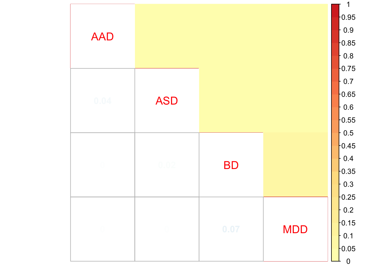

Expand here to see past versions of unnamed-chunk-9-1.png:

Version	Author	Date
4a8a857	zouyuxin	2018-05-12

Session information

sessionInfo()

R version 3.4.4 (2018-03-15)
Platform: x86_64-apple-darwin15.6.0 (64-bit)
Running under: macOS High Sierra 10.13.4

Matrix products: default
BLAS: /Library/Frameworks/R.framework/Versions/3.4/Resources/lib/libRblas.0.dylib
LAPACK: /Library/Frameworks/R.framework/Versions/3.4/Resources/lib/libRlapack.dylib

locale:
[1] en_US.UTF-8/en_US.UTF-8/en_US.UTF-8/C/en_US.UTF-8/en_US.UTF-8

attached base packages:
[1] stats     graphics  grDevices utils     datasets  methods   base     

other attached packages:
[1] corrplot_0.84  colorRamps_2.3 flashr_0.5-6   plyr_1.8.4    
[5] mclust_5.4     mashr_0.2-8    ashr_2.2-7     limma_3.34.9  

loaded via a namespace (and not attached):
 [1] Rcpp_0.12.16      pillar_1.2.2      compiler_3.4.4   
 [4] git2r_0.21.0      workflowr_1.0.1   R.methodsS3_1.7.1
 [7] R.utils_2.6.0     iterators_1.0.9   tools_3.4.4      
[10] digest_0.6.15     tibble_1.4.2      gtable_0.2.0     
[13] evaluate_0.10.1   lattice_0.20-35   rlang_0.2.0      
[16] Matrix_1.2-14     foreach_1.4.4     yaml_2.1.19      
[19] parallel_3.4.4    mvtnorm_1.0-7     ebnm_0.1-11      
[22] stringr_1.3.0     knitr_1.20        REBayes_1.3      
[25] rprojroot_1.3-2   grid_3.4.4        rmarkdown_1.9    
[28] rmeta_3.0         ggplot2_2.2.1     magrittr_1.5     
[31] whisker_0.3-2     scales_0.5.0      backports_1.1.2  
[34] codetools_0.2-15  htmltools_0.3.6   MASS_7.3-50      
[37] assertthat_0.2.0  softImpute_1.4    colorspace_1.3-2 
[40] stringi_1.2.2     Rmosek_8.0.69     lazyeval_0.2.1   
[43] munsell_0.4.3     doParallel_1.0.11 pscl_1.5.2       
[46] truncnorm_1.0-8   SQUAREM_2017.10-1 R.oo_1.22.0

This reproducible R Markdown analysis was created with workflowr 1.0.1