susie z from logistic regression
Yuxin Zou
2018-12-4
Last updated: 2018-12-10
workflowr checks: (Click a bullet for more information)-
✔ R Markdown file: up-to-date
Great! Since the R Markdown file has been committed to the Git repository, you know the exact version of the code that produced these results.
-
✔ Environment: empty
Great job! The global environment was empty. Objects defined in the global environment can affect the analysis in your R Markdown file in unknown ways. For reproduciblity it’s best to always run the code in an empty environment.
-
✔ Seed:
set.seed(20180529)The command
set.seed(20180529)was run prior to running the code in the R Markdown file. Setting a seed ensures that any results that rely on randomness, e.g. subsampling or permutations, are reproducible. -
✔ Session information: recorded
Great job! Recording the operating system, R version, and package versions is critical for reproducibility.
-
Great! You are using Git for version control. Tracking code development and connecting the code version to the results is critical for reproducibility. The version displayed above was the version of the Git repository at the time these results were generated.✔ Repository version: f5995ef
Note that you need to be careful to ensure that all relevant files for the analysis have been committed to Git prior to generating the results (you can usewflow_publishorwflow_git_commit). workflowr only checks the R Markdown file, but you know if there are other scripts or data files that it depends on. Below is the status of the Git repository when the results were generated:
Note that any generated files, e.g. HTML, png, CSS, etc., are not included in this status report because it is ok for generated content to have uncommitted changes.Ignored files: Ignored: .Rhistory Ignored: .Rproj.user/ Ignored: analysis/.Rhistory Ignored: docs/.DS_Store Ignored: docs/figure/Test.Rmd/ Ignored: output/MASHbaselineFigures/ Untracked files: Untracked: analysis/DifferentCovModel.Rmd Untracked: analysis/MASH_est_Cor.Rmd Untracked: analysis/MASHbaselineCode.Rmd Untracked: analysis/MashEstCorProblem.Rmd Untracked: analysis/MashMedian.Rmd Untracked: analysis/mashMean.Rmd Untracked: code/DifferentCov.R Untracked: code/EstCorV.R Untracked: code/generateDataV.R Untracked: code/summary.R Untracked: docs/Estimate_Null_Cor_New.pdf Untracked: docs/Estimate_Null_Cor_Old.pdf Untracked: output/MASH.result.1.rds Untracked: output/MASH.result.10.rds Untracked: output/MASH.result.2.rds Untracked: output/MASH.result.3.rds Untracked: output/MASH.result.4.rds Untracked: output/MASH.result.5.rds Untracked: output/MASH.result.6.rds Untracked: output/MASH.result.7.rds Untracked: output/MASH.result.8.rds Untracked: output/MASH.result.9.rds Unstaged changes: Modified: analysis/susieProblem2.Rmd
Expand here to see past versions:
| File | Version | Author | Date | Message |
|---|---|---|---|---|
| Rmd | f5995ef | zouyuxin | 2018-12-10 | wflow_publish(“analysis/susieZBinary.Rmd”) |
| html | 003188b | zouyuxin | 2018-12-10 | Build site. |
| Rmd | d9efc36 | zouyuxin | 2018-12-10 | wflow_publish(“analysis/susieZBinary.Rmd”) |
| html | cb3f4e5 | zouyuxin | 2018-12-05 | Build site. |
| Rmd | b371cf8 | zouyuxin | 2018-12-05 | wflow_publish(“analysis/susieZBinary.Rmd”) |
| html | 213b965 | zouyuxin | 2018-12-04 | Build site. |
| Rmd | 7fa45bb | zouyuxin | 2018-12-04 | wflow_publish(“analysis/susieZBinary.Rmd”) |
We show the performance of susie z when the z scores come from logistic regression.
When sample size n is large and greater than p, the susie model captures some causal effects. When n less than p, the susie model fails to find any causal effect sometimes.
library(susieR)Simulation: X independent
n \(>\) p
We run similations with n > p. Let n = 1000, p=500. The susie model captures the true effects in all cases below.
- Case 1: L=1. The true effect is b200. The response y is simulated from the specified bernoulli model without intercept, which means the number of case-control is well-balanced. The susie model captures the causal effect.
set.seed(1)
n = 1000
p = 500

X = matrix(rnorm(n*p, 0, 1), nrow = n, ncol = p)
R = cor(X)
beta_true = rep(0, p)
beta_true[200] = 1
Y = rbinom(n, 1, exp(X %*% beta_true) / (1 + exp(X %*% beta_true)))
z = numeric(p)
for(i in 1:p){
z[i] = summary(glm(Y~X[,i], family = 'binomial'))$coef[2,3]
}susie_plot(z, y='z', b=beta_true)
Expand here to see past versions of unnamed-chunk-4-1.png:
| Version | Author | Date |
|---|---|---|
| 003188b | zouyuxin | 2018-12-10 |
| 213b965 | zouyuxin | 2018-12-04 |
fit_z = susieR::susie_z(z, R, min_abs_corr = 0)susie_plot(fit_z, y="PIP", b=beta_true)
Expand here to see past versions of unnamed-chunk-6-1.png:
| Version | Author | Date |
|---|---|---|
| 003188b | zouyuxin | 2018-12-10 |
| cb3f4e5 | zouyuxin | 2018-12-05 |
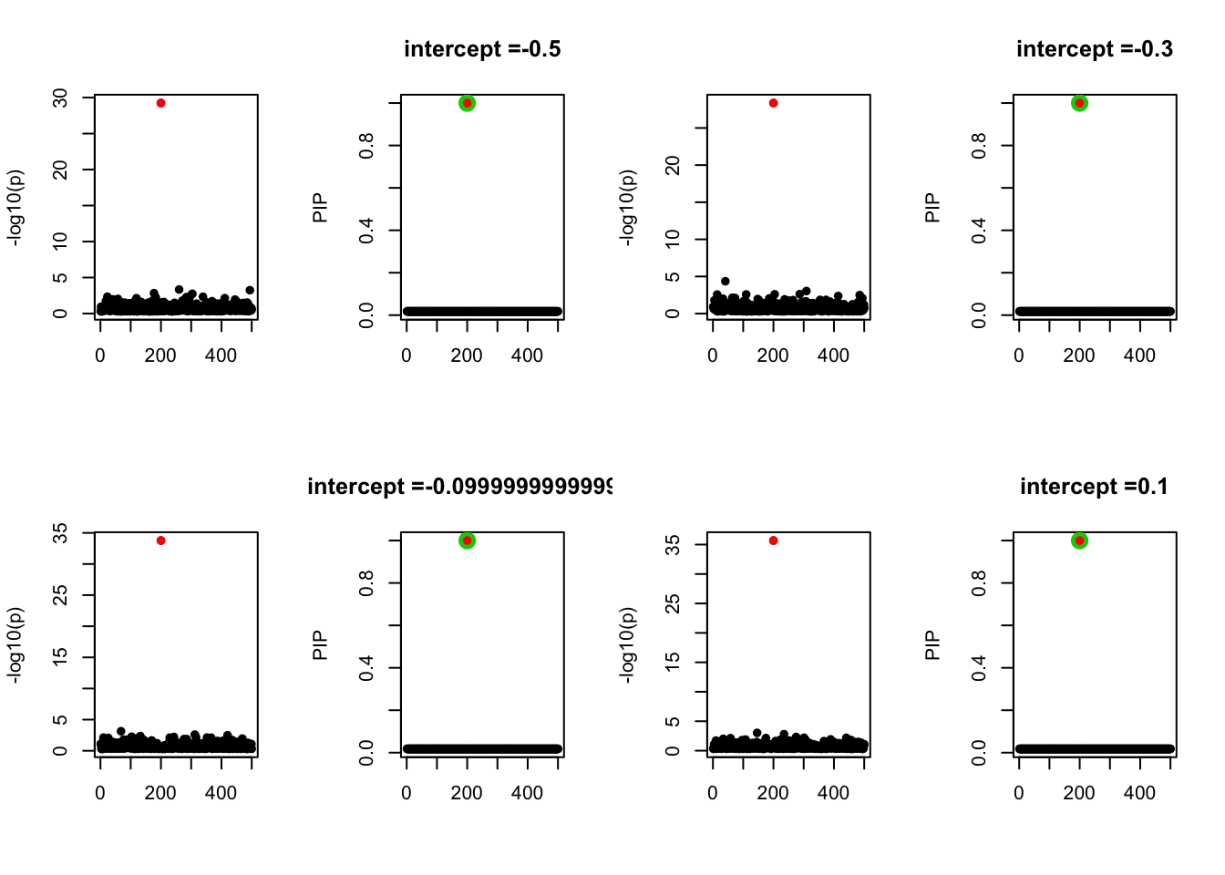
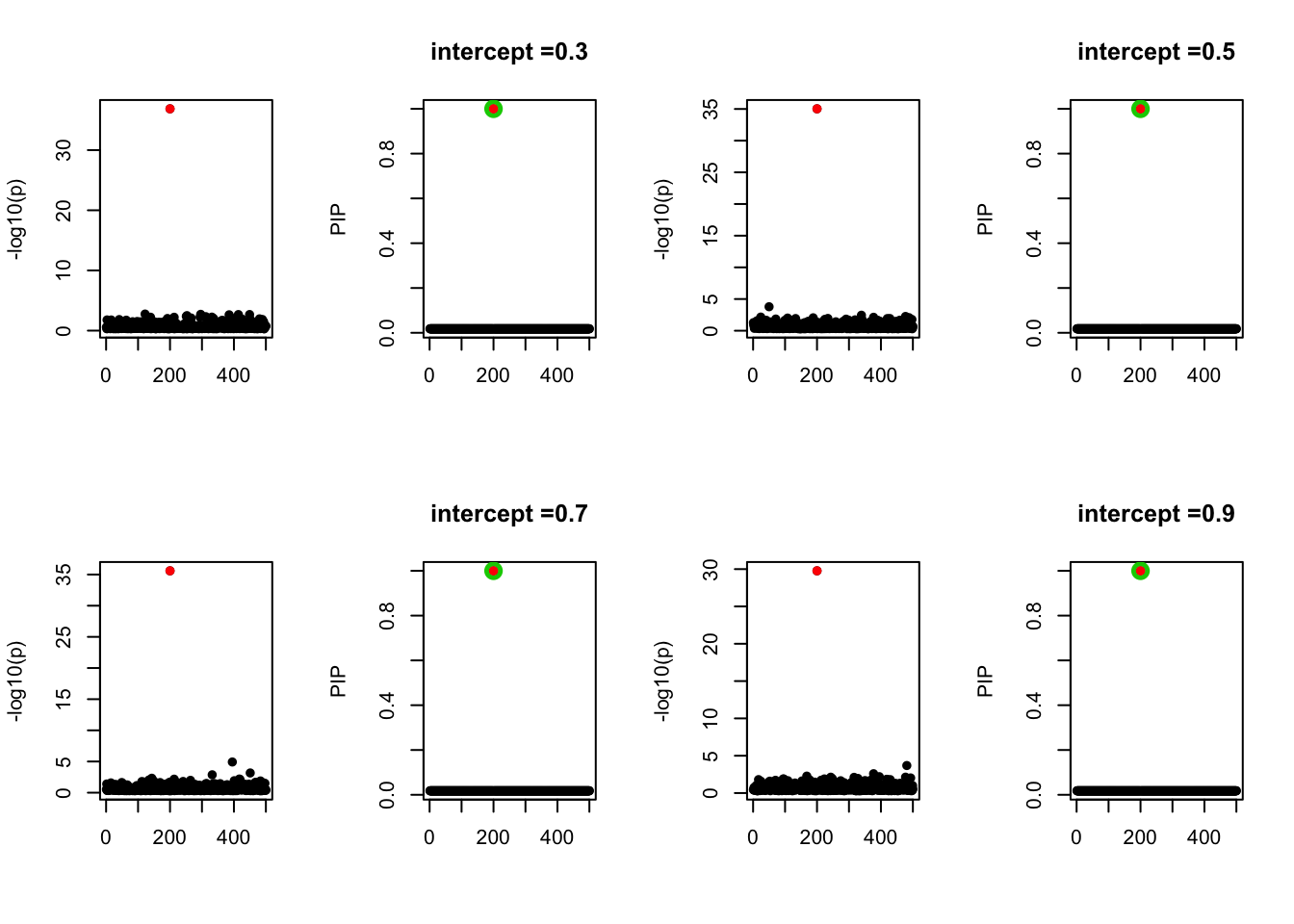
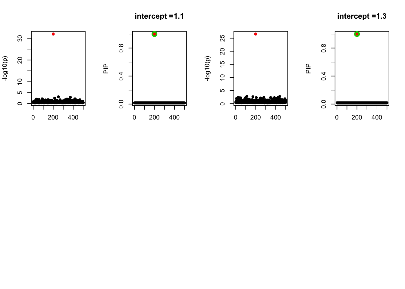
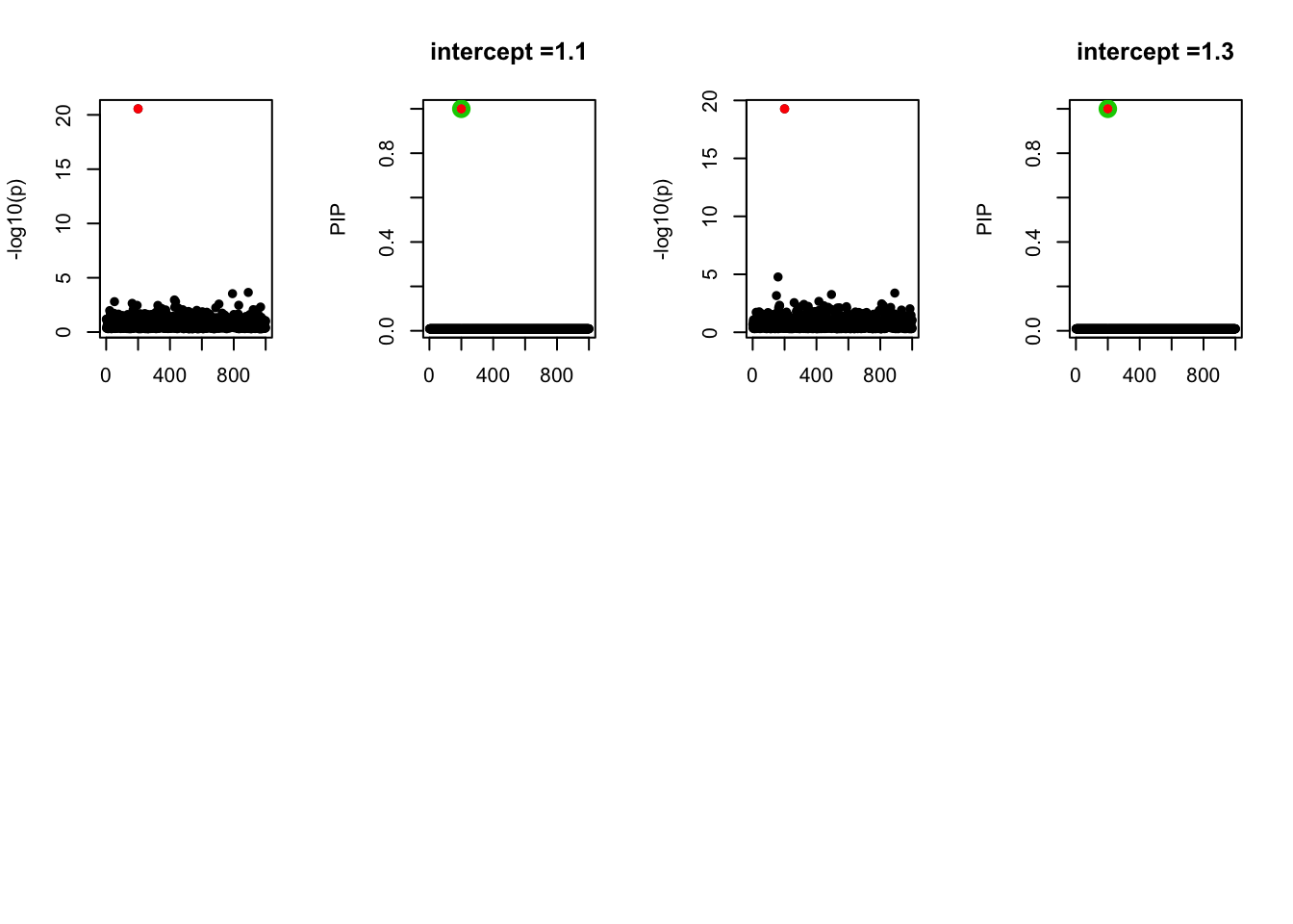
- Case 2: The response y is simulated from the specified bernoulli model with intercept from -1.3 to 1.3. When the intercept is not zero, the case-control is not balanced. The susie model captures the causal effect.
par(mfrow=c(2, 4))
alpha = seq(-1.3,1.3,by=0.2)
set.seed(1)
for(a in alpha){
  Y = rbinom(n, 1, exp(a+X %*% beta_true) / (1 + exp(a+X %*% beta_true)))

  z = numeric(p)
  for(i in 1:p){
    z[i] = summary(glm(Y~X[,i], family = 'binomial'))$coef[2,3]
  }
  susie_plot(z, y='z', b=beta_true)
  fit_z = susieR::susie_z(z, R, min_abs_corr = 0)
  susie_plot(fit_z, y="PIP", b=beta_true, main=paste0('intercept =', a))
}
Expand here to see past versions of unnamed-chunk-7-1.png:
| Version | Author | Date |
|---|---|---|
| 003188b | zouyuxin | 2018-12-10 |
| 213b965 | zouyuxin | 2018-12-04 |
Expand here to see past versions of unnamed-chunk-7-2.png:
| Version | Author | Date |
|---|---|---|
| 003188b | zouyuxin | 2018-12-10 |
Expand here to see past versions of unnamed-chunk-7-3.png:
| Version | Author | Date |
|---|---|---|
| 003188b | zouyuxin | 2018-12-10 |
Expand here to see past versions of unnamed-chunk-7-4.png:
| Version | Author | Date |
|---|---|---|
| 003188b | zouyuxin | 2018-12-10 |
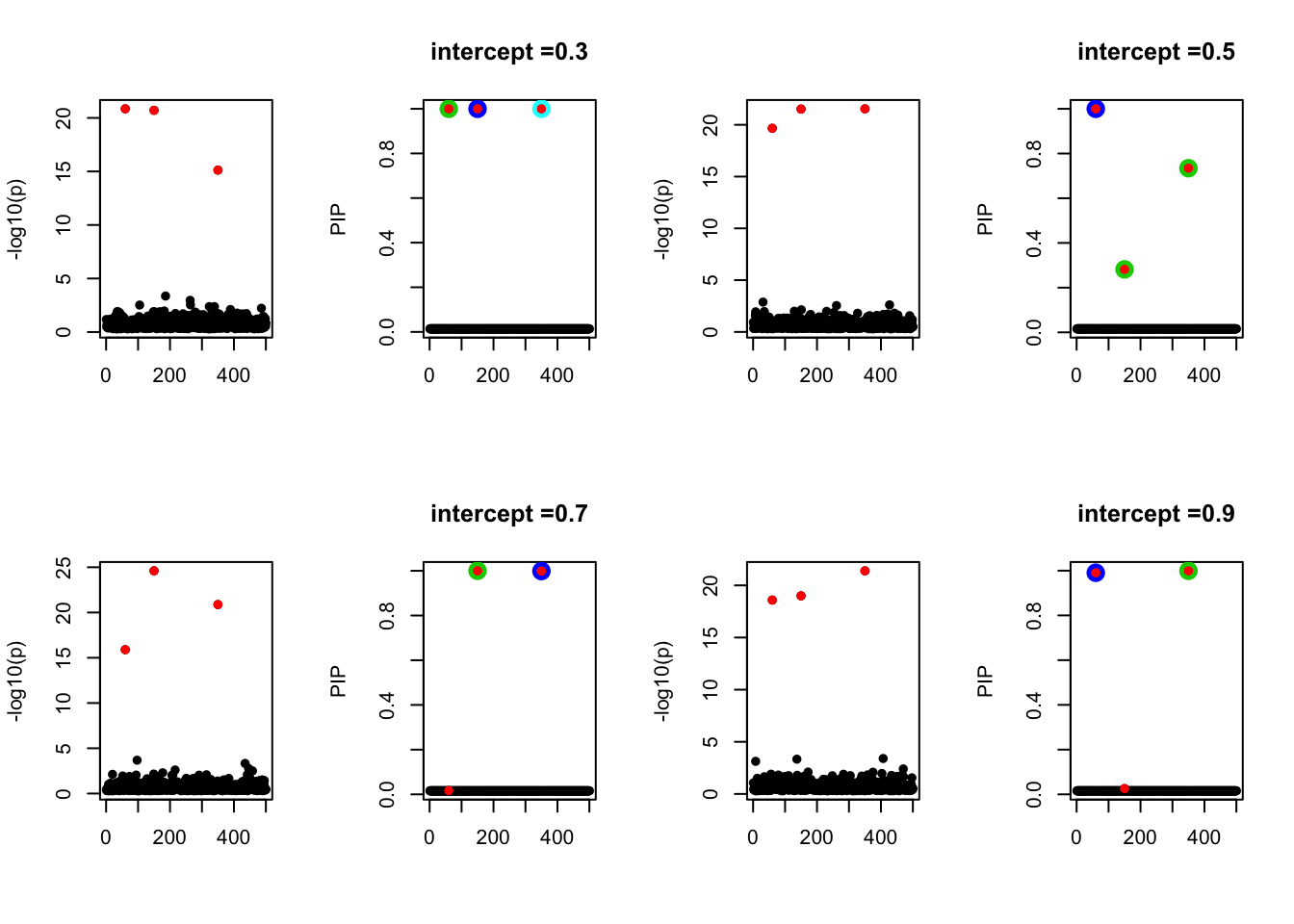
- Case 3: We increase the number of true effects to be 3. The true effects are b60, b150, b350. The response y is simulated from the specified bernoulli model without intercept. The susie model captures 2 causal effects.
beta_true = rep(0, p)
beta_true[c(60,350)] = 1
beta_true[150] = -1
set.seed(1)
Y = rbinom(n, 1, exp(X %*% beta_true) / (1 + exp(X %*% beta_true)))

z = numeric(p)
for(i in 1:p){
  z[i] = summary(glm(Y~X[,i], family = 'binomial'))$coef[2,3]
}

susie_plot(z, y='z', b=beta_true)
Expand here to see past versions of unnamed-chunk-8-1.png:
| Version | Author | Date |
|---|---|---|
| 003188b | zouyuxin | 2018-12-10 |
| cb3f4e5 | zouyuxin | 2018-12-05 |
fit_z = susieR::susie_z(z, R, min_abs_corr = 0)susie_plot(fit_z, y="PIP", b=beta_true)
Expand here to see past versions of unnamed-chunk-9-1.png:
| Version | Author | Date |
|---|---|---|
| 003188b | zouyuxin | 2018-12-10 |
| cb3f4e5 | zouyuxin | 2018-12-05 |
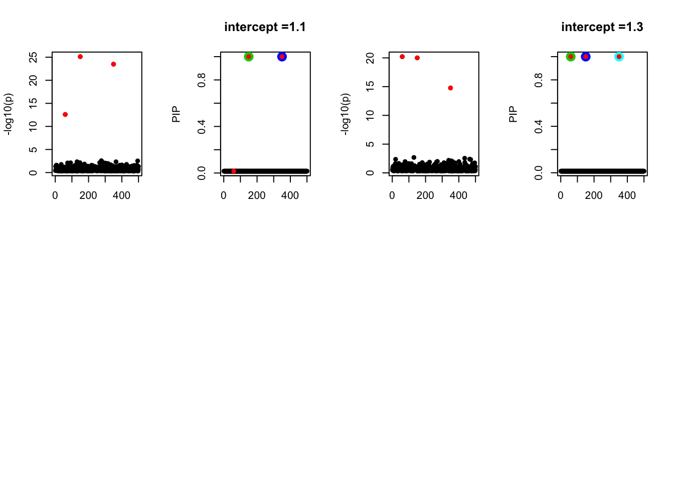
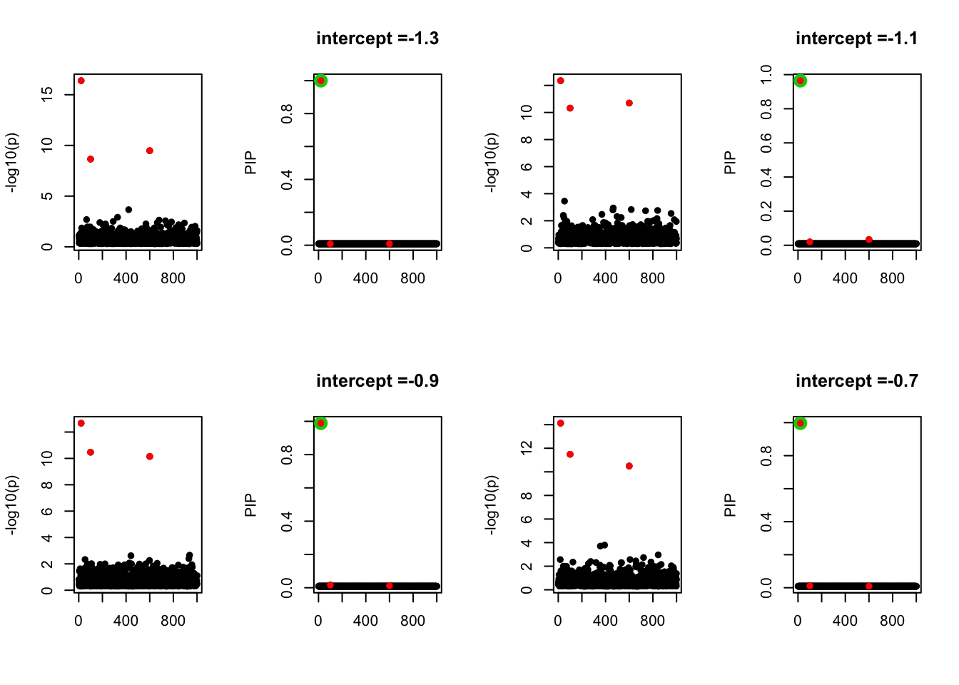
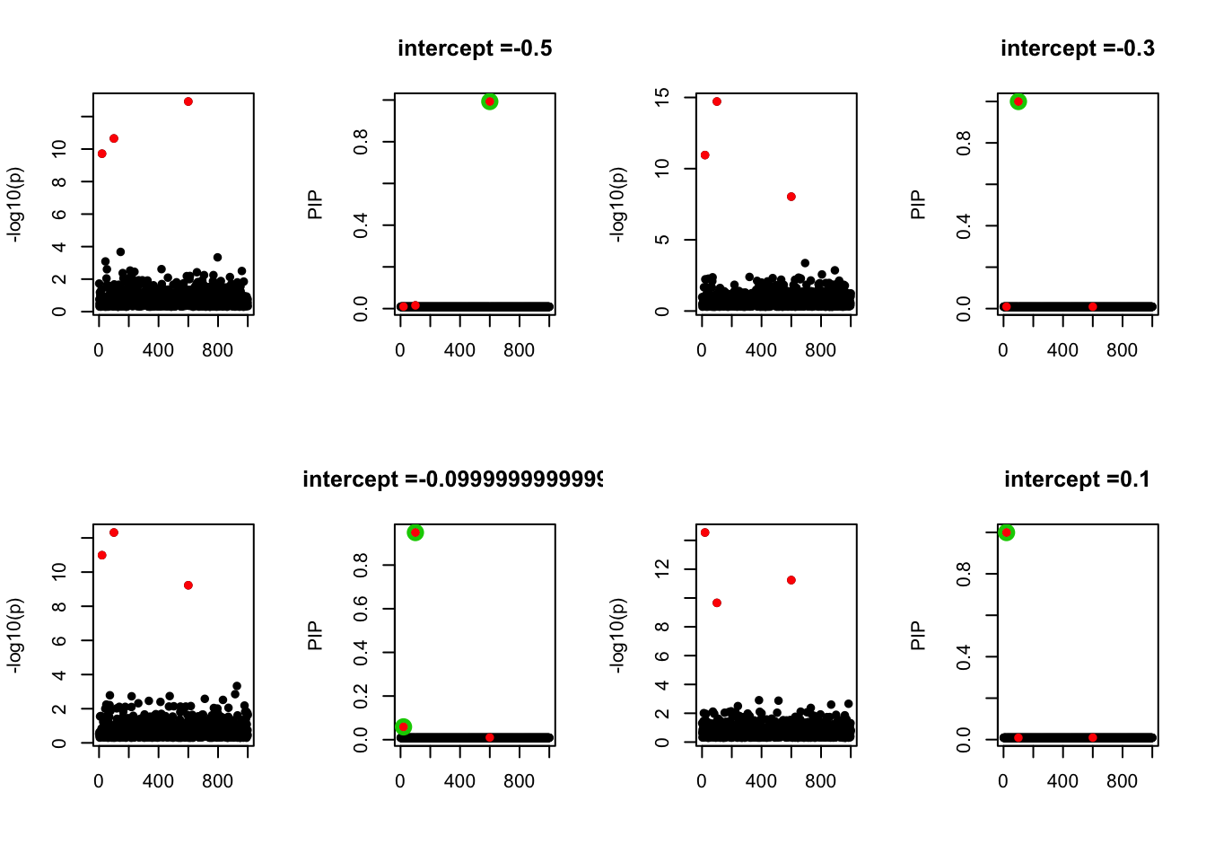
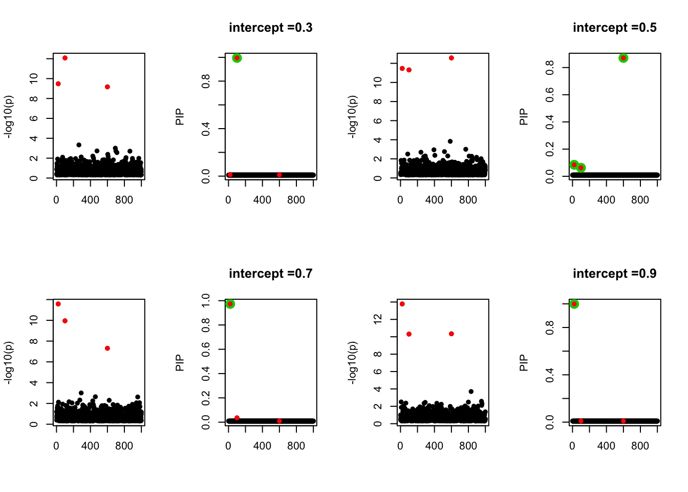
- Case 4: The number of true effects is 3 and the response y is simulated from the specified bernoulli model with intercept from -1.3 to 1.3.
par(mfrow=c(2, 4))
alpha = seq(-1.3,1.3,by=0.2)
set.seed(1)
for(a in alpha){
  Y = rbinom(n, 1, exp(a+X %*% beta_true) / (1 + exp(a+X %*% beta_true)))

  z = numeric(p)
  for(i in 1:p){
    z[i] = summary(glm(Y~X[,i], family = 'binomial'))$coef[2,3]
  }
  susie_plot(z, y='z', b=beta_true)
  fit_z = susieR::susie_z(z, R, min_abs_corr = 0)
  susie_plot(fit_z, y="PIP", b=beta_true, main=paste0('intercept =', a))
}
Expand here to see past versions of unnamed-chunk-10-1.png:
| Version | Author | Date |
|---|---|---|
| 003188b | zouyuxin | 2018-12-10 |
Expand here to see past versions of unnamed-chunk-10-2.png:
| Version | Author | Date |
|---|---|---|
| 003188b | zouyuxin | 2018-12-10 |
Expand here to see past versions of unnamed-chunk-10-3.png:
| Version | Author | Date |
|---|---|---|
| 003188b | zouyuxin | 2018-12-10 |
Expand here to see past versions of unnamed-chunk-10-4.png:
| Version | Author | Date |
|---|---|---|
| 003188b | zouyuxin | 2018-12-10 |
n \(<\) p
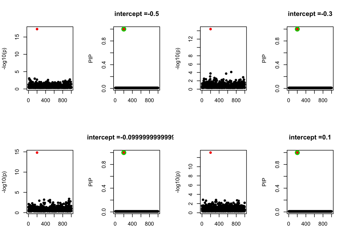
We run similations with n < p. Let n = 500, p=1000. The susie model does not capture the causal effects in all cases below.
- Case 1: L=1. The true effect is b200. The response y is simulated from the specified bernoulli model without intercept.
set.seed(1)
n = 500
p = 1000

beta_true = rep(0, p)
beta_true[200] = 1

X = matrix(rnorm(n*p, 0, 1), nrow = n, ncol = p)
R = cor(X)

Y = rbinom(n, 1, exp(X %*% beta_true) / (1 + exp(X %*% beta_true)))

z = numeric(p)
for(i in 1:p){
  z[i] = summary(glm(Y~X[,i], family = 'binomial'))$coef[2,3]
}
susie_plot(z, y='z', b=beta_true)
Expand here to see past versions of unnamed-chunk-12-1.png:
| Version | Author | Date |
|---|---|---|
| 003188b | zouyuxin | 2018-12-10 |
| cb3f4e5 | zouyuxin | 2018-12-05 |
fit_z = susieR::susie_z(z, R, min_abs_corr = 0)susie_plot(fit_z, y="PIP", b=beta_true)
Expand here to see past versions of unnamed-chunk-14-1.png:
| Version | Author | Date |
|---|---|---|
| 003188b | zouyuxin | 2018-12-10 |
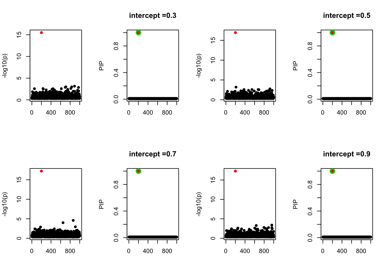
- Case 2: The response y is simulated from the specified bernoulli model with intercept from -1.3 to 1.3.
par(mfrow=c(2, 4))
alpha = seq(-1.3,1.3,by=0.2)
set.seed(1)
for(a in alpha){
  Y = rbinom(n, 1, exp(a+X %*% beta_true) / (1 + exp(a+X %*% beta_true)))

  z = numeric(p)
  for(i in 1:p){
    z[i] = summary(glm(Y~X[,i], family = 'binomial'))$coef[2,3]
  }
  susie_plot(z, y='z', b=beta_true)
  fit_z = susieR::susie_z(z, R, min_abs_corr = 0)
  susie_plot(fit_z, y="PIP", b=beta_true, main=paste0('intercept =', a))
}
Expand here to see past versions of unnamed-chunk-15-1.png:
| Version | Author | Date |
|---|---|---|
| 003188b | zouyuxin | 2018-12-10 |
| cb3f4e5 | zouyuxin | 2018-12-05 |
Expand here to see past versions of unnamed-chunk-15-2.png:
| Version | Author | Date |
|---|---|---|
| 003188b | zouyuxin | 2018-12-10 |
Expand here to see past versions of unnamed-chunk-15-3.png:
| Version | Author | Date |
|---|---|---|
| 003188b | zouyuxin | 2018-12-10 |
Expand here to see past versions of unnamed-chunk-15-4.png:
| Version | Author | Date |
|---|---|---|
| 003188b | zouyuxin | 2018-12-10 |
- Case 3: The number of true effects is 3. The true effects are b20, b100, b600. The response y is simulated from the specified bernoulli model without intercept.
beta_true = rep(0, p)
beta_true[c(20,600)] = 1
beta_true[100] = -1
set.seed(1)
Y = rbinom(n, 1, exp(X %*% beta_true) / (1 + exp(X %*% beta_true)))

z = numeric(p)
for(i in 1:p){
  z[i] = summary(glm(Y~X[,i], family = 'binomial'))$coef[2,3]
}
susie_plot(z, y='z', b=beta_true)
Expand here to see past versions of unnamed-chunk-16-1.png:
| Version | Author | Date |
|---|---|---|
| 003188b | zouyuxin | 2018-12-10 |
| cb3f4e5 | zouyuxin | 2018-12-05 |
fit_z = susieR::susie_z(z, R, min_abs_corr = 0)susie_plot(fit_z, y="PIP", b=beta_true)
Expand here to see past versions of unnamed-chunk-17-1.png:
| Version | Author | Date |
|---|---|---|
| 003188b | zouyuxin | 2018-12-10 |
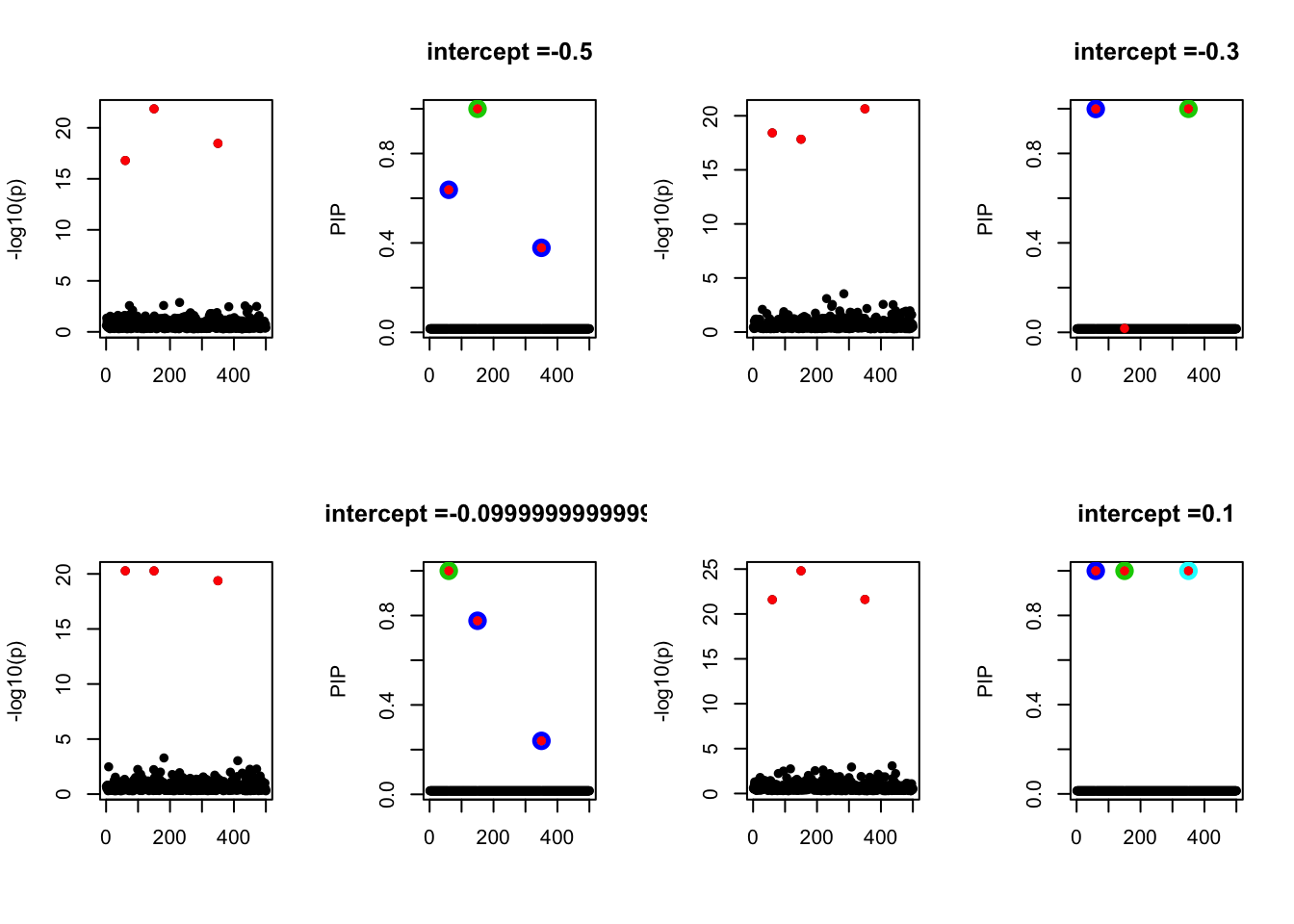
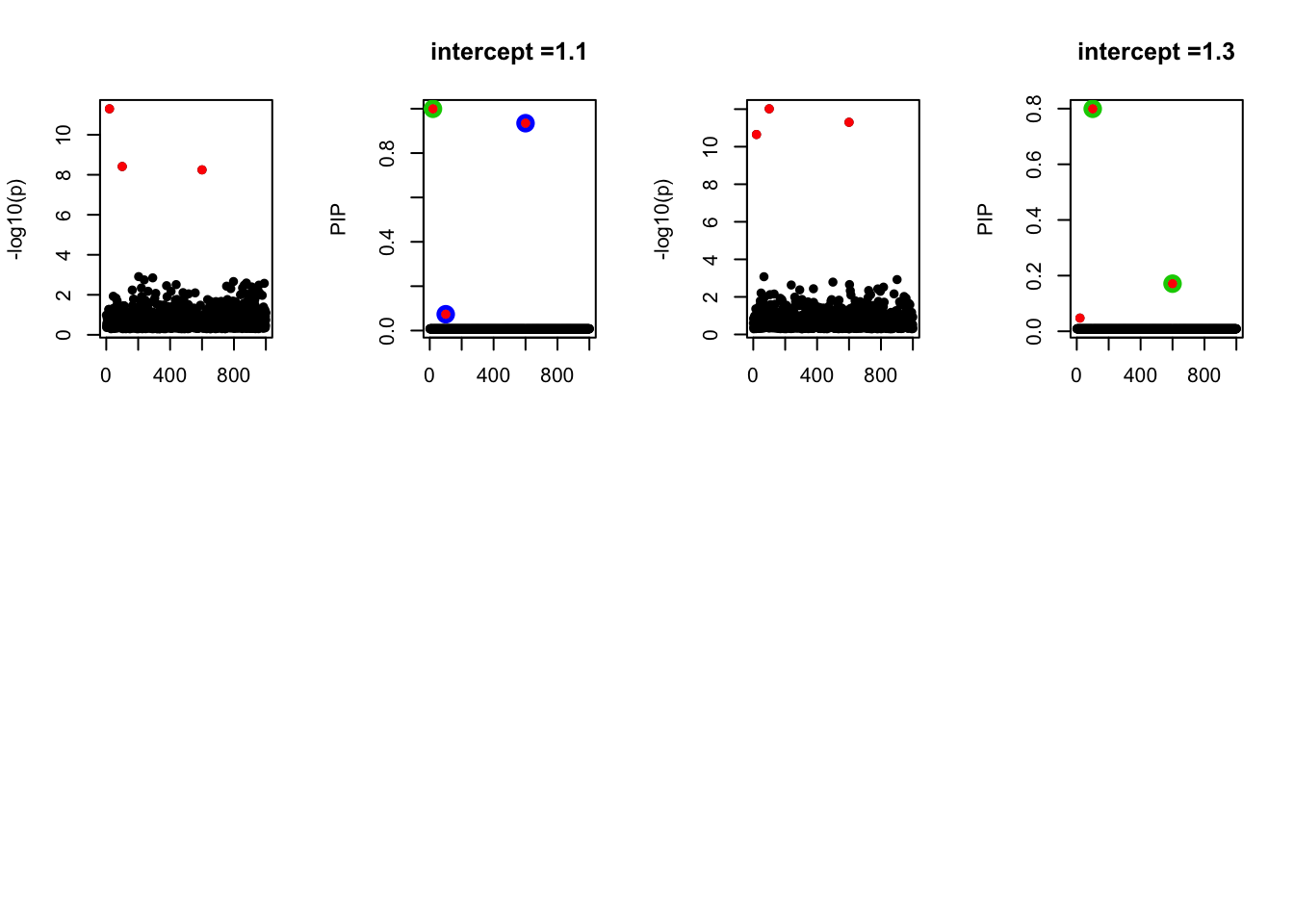
- Case 4: The number of true effects is 3 and the response y is simulated from the specified bernoulli model with intercept from -1.3 to 1.3.
par(mfrow=c(2, 4))
alpha = seq(-1.3,1.3,by=0.2)
set.seed(1)
for(a in alpha){
  Y = rbinom(n, 1, exp(a+X %*% beta_true) / (1 + exp(a+X %*% beta_true)))

  z = numeric(p)
  for(i in 1:p){
    z[i] = summary(glm(Y~X[,i], family = 'binomial'))$coef[2,3]
  }
  susie_plot(z, y='z', b=beta_true)
  fit_z = susieR::susie_z(z, R, min_abs_corr = 0)
  susie_plot(fit_z, y="PIP", b=beta_true, main=paste0('intercept =', a))
}
Expand here to see past versions of unnamed-chunk-18-1.png:
| Version | Author | Date |
|---|---|---|
| 003188b | zouyuxin | 2018-12-10 |
| cb3f4e5 | zouyuxin | 2018-12-05 |
Expand here to see past versions of unnamed-chunk-18-2.png:
| Version | Author | Date |
|---|---|---|
| 003188b | zouyuxin | 2018-12-10 |
Expand here to see past versions of unnamed-chunk-18-3.png:
| Version | Author | Date |
|---|---|---|
| 003188b | zouyuxin | 2018-12-10 |
Expand here to see past versions of unnamed-chunk-18-4.png:
| Version | Author | Date |
|---|---|---|
| 003188b | zouyuxin | 2018-12-10 |
Simulation: X correlated
The data X is from the susie pacakge, ‘N3finemapping’. There are 3 true effects.
data(N3finemapping)
attach(N3finemapping)
X = data$X
b <- data$true_coef[,1]
The true effects are
plot(b, pch=16, ylab='effect size')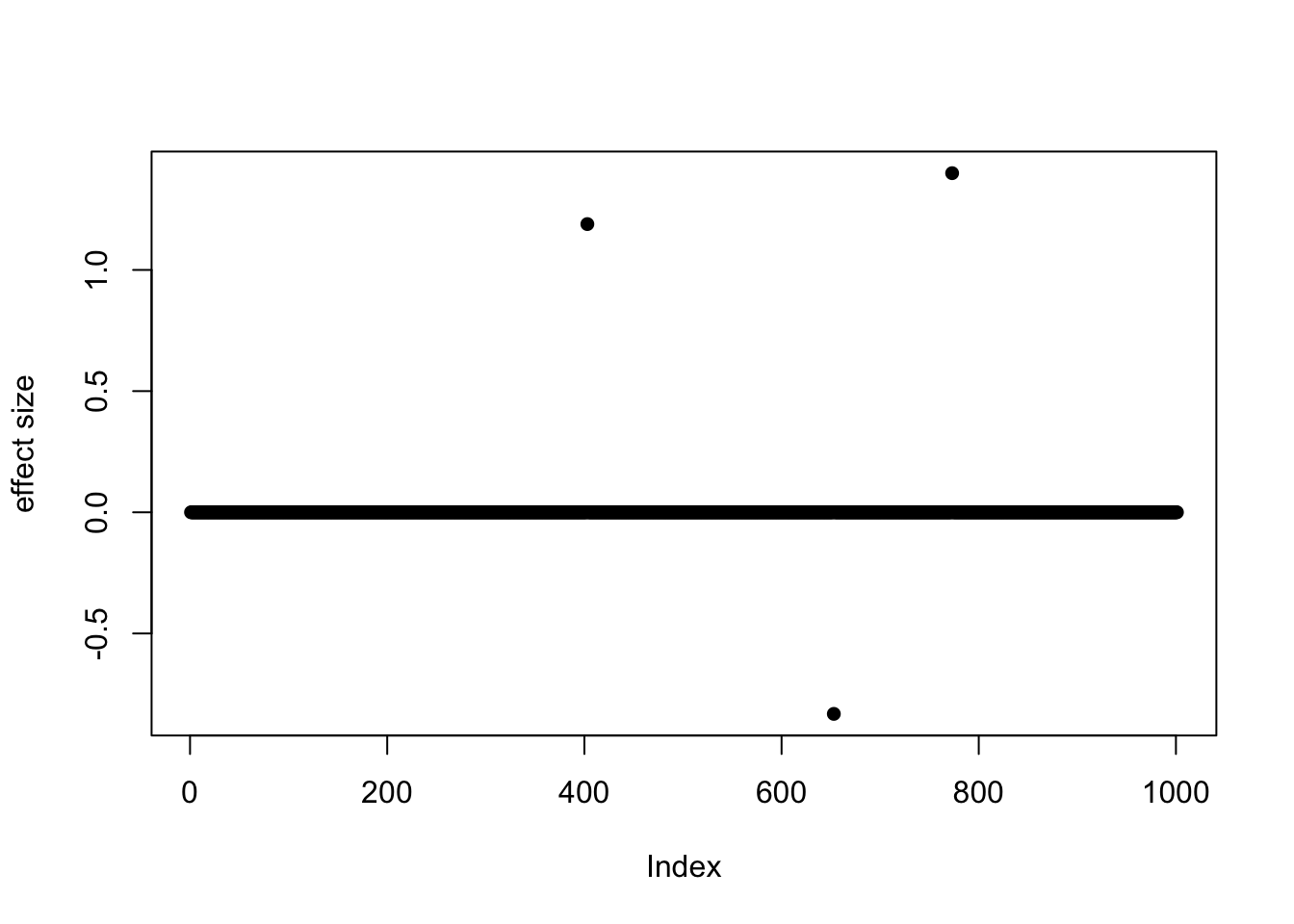
Expand here to see past versions of unnamed-chunk-20-1.png:
| Version | Author | Date |
|---|---|---|
| 003188b | zouyuxin | 2018-12-10 |
| cb3f4e5 | zouyuxin | 2018-12-05 |
We simulate y from the specified bernoulli model without intercept.
set.seed(201812)
y = rbinom(nrow(X), 1, exp(X %*% b) / (1 + exp(X %*% b)))
z = numeric(length(b))
for(i in 1:length(b)){
  z[i] = summary(glm(y~X[,i], family = 'binomial'))$coef[2,3]
}
R = cor(X)
susie_plot(z, y='z', b=b)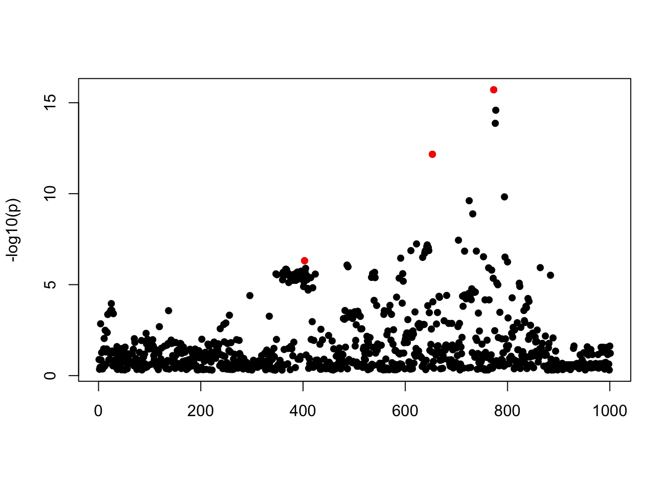
Expand here to see past versions of unnamed-chunk-21-1.png:
| Version | Author | Date |
|---|---|---|
| 003188b | zouyuxin | 2018-12-10 |
| cb3f4e5 | zouyuxin | 2018-12-05 |
fit_z = susieR::susie_z(z, R, min_abs_corr = 0)susie_plot(fit_z, y="PIP", b=b)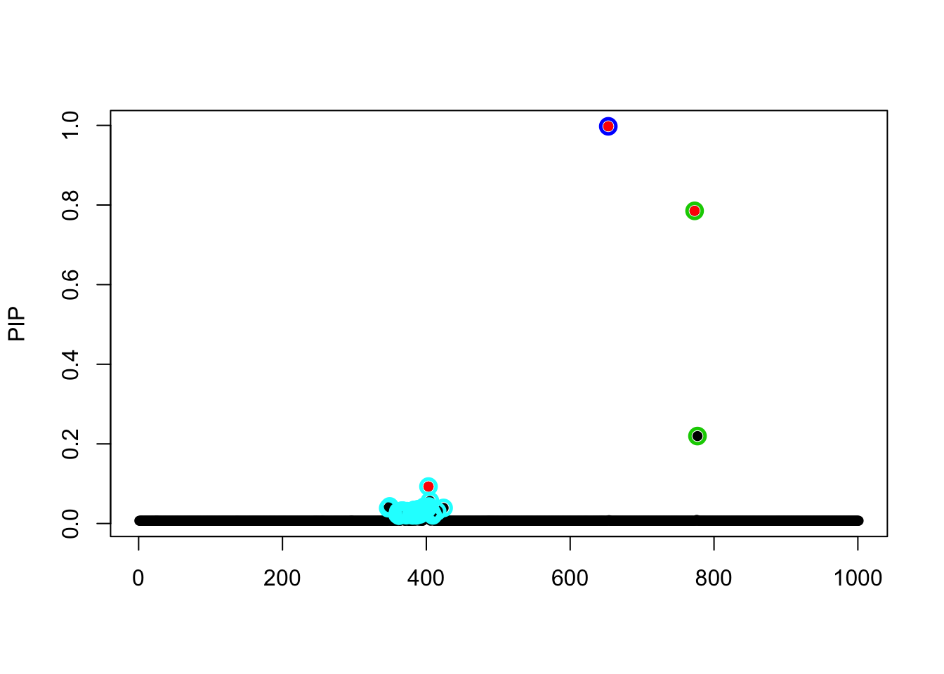
Expand here to see past versions of unnamed-chunk-22-1.png:
| Version | Author | Date |
|---|---|---|
| 003188b | zouyuxin | 2018-12-10 |
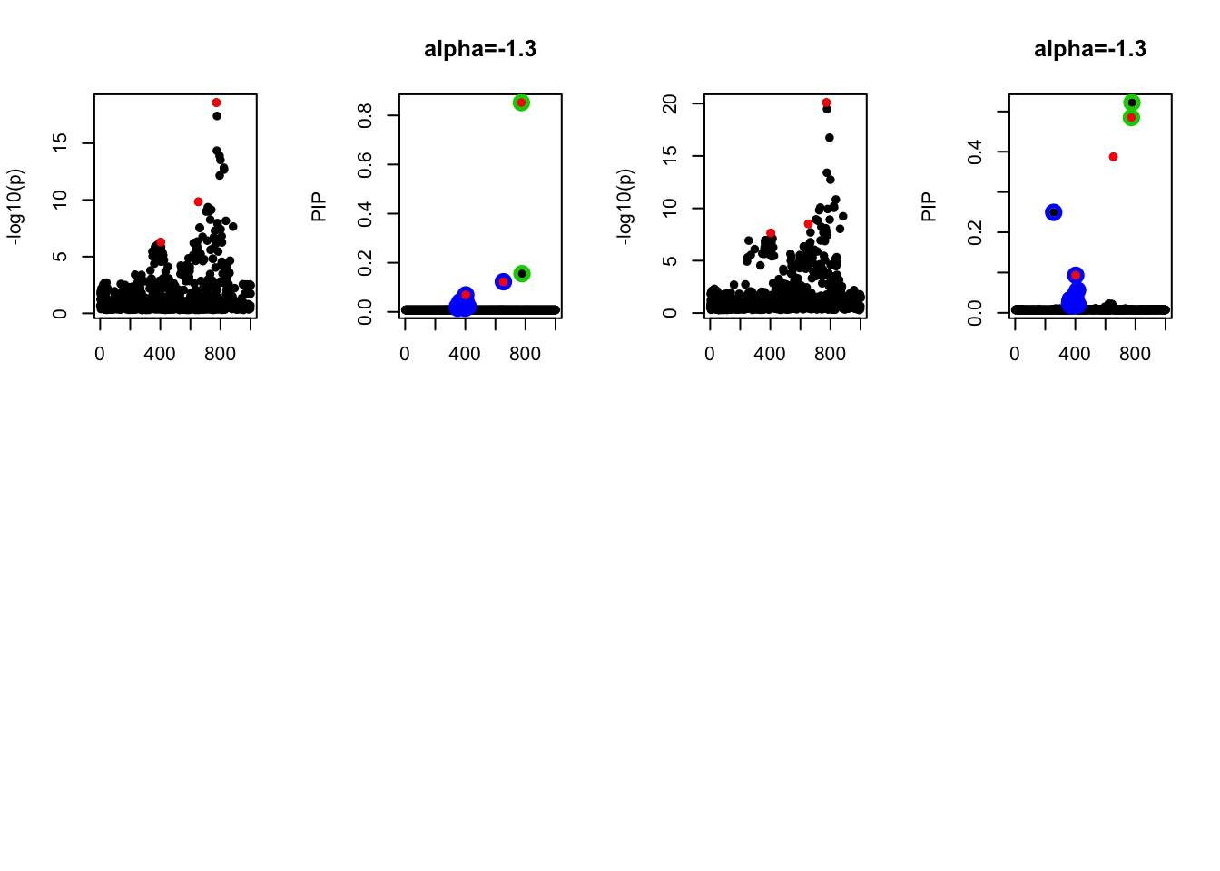
We simulate y with different intercept value.
par(mfrow=c(2,4))
set.seed(2018)
alpha = seq(-1.3,1.3,by=0.2)
for(a in alpha){
  a = -1.3
  y = rbinom(nrow(X), 1, exp(a+X %*% b) / (1 + exp(a+X %*% b)))
  z = numeric(length(b))
  for(i in 1:length(b)){
    # m = withCallingHandlers(glm(y~X[,i], family = 'binomial'), warning = function(w) {
    #                   if (grepl("fitted probabilities", w$message)){
    #                     print(i)
    #                   }
    #                 })
    m = glm(y~X[,i], family = 'binomial')
    z[i] = summary(m)$coef[2,3]
  }
  susie_plot(z, y='z', b=b)
  fit_z = susieR::susie_z(z, R, min_abs_corr = 0)
  susie_plot(fit_z, y="PIP", b=b, main=paste0('alpha=', a))
}
Warning: glm.fit: fitted probabilities numerically 0 or 1 occurred
Warning: glm.fit: fitted probabilities numerically 0 or 1 occurred
Warning: glm.fit: fitted probabilities numerically 0 or 1 occurred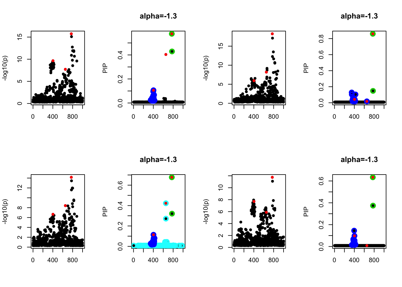
Expand here to see past versions of unnamed-chunk-23-1.png:
| Version | Author | Date |
|---|---|---|
| 003188b | zouyuxin | 2018-12-10 |
Warning: glm.fit: fitted probabilities numerically 0 or 1 occurred
Warning: glm.fit: fitted probabilities numerically 0 or 1 occurred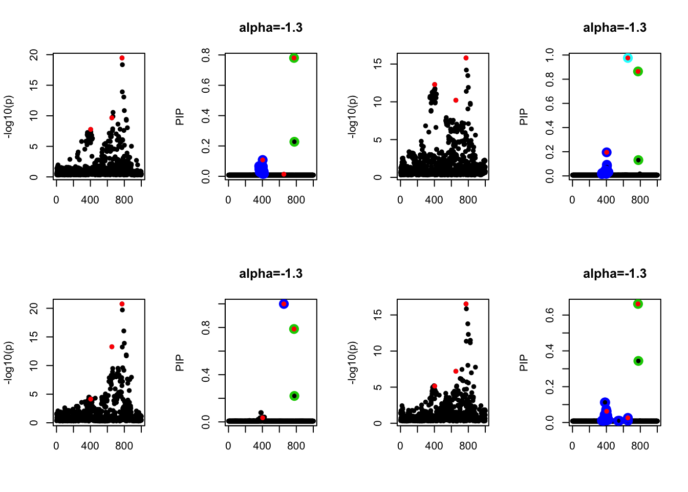
Expand here to see past versions of unnamed-chunk-23-2.png:
| Version | Author | Date |
|---|---|---|
| 003188b | zouyuxin | 2018-12-10 |
Warning: glm.fit: fitted probabilities numerically 0 or 1 occurred

Warning: glm.fit: fitted probabilities numerically 0 or 1 occurred

Warning: glm.fit: fitted probabilities numerically 0 or 1 occurred
Warning: glm.fit: fitted probabilities numerically 0 or 1 occurred

Warning: glm.fit: fitted probabilities numerically 0 or 1 occurred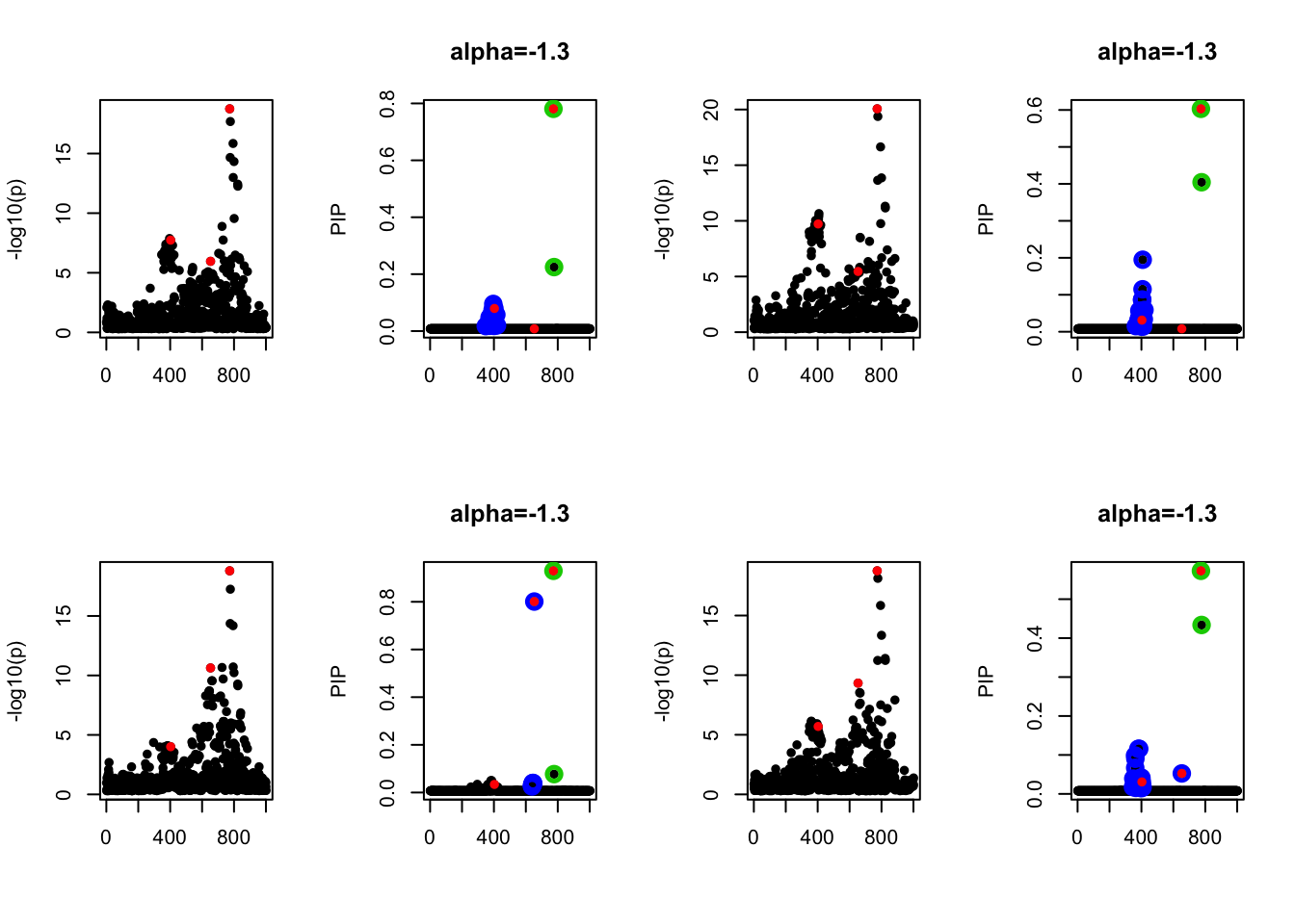
Expand here to see past versions of unnamed-chunk-23-3.png:
| Version | Author | Date |
|---|---|---|
| 003188b | zouyuxin | 2018-12-10 |
Expand here to see past versions of unnamed-chunk-23-4.png:
| Version | Author | Date |
|---|---|---|
| 003188b | zouyuxin | 2018-12-10 |
Session information
sessionInfo()R version 3.5.1 (2018-07-02)
Platform: x86_64-apple-darwin15.6.0 (64-bit)
Running under: macOS 10.14.1
Matrix products: default
BLAS: /Library/Frameworks/R.framework/Versions/3.5/Resources/lib/libRblas.0.dylib
LAPACK: /Library/Frameworks/R.framework/Versions/3.5/Resources/lib/libRlapack.dylib
locale:
[1] en_US.UTF-8/en_US.UTF-8/en_US.UTF-8/C/en_US.UTF-8/en_US.UTF-8
attached base packages:
[1] stats graphics grDevices utils datasets methods base
other attached packages:
[1] susieR_0.6.2.0405
loaded via a namespace (and not attached):
[1] workflowr_1.1.1 Rcpp_1.0.0 lattice_0.20-35
[4] digest_0.6.18 rprojroot_1.3-2 R.methodsS3_1.7.1
[7] grid_3.5.1 backports_1.1.2 magrittr_1.5
[10] git2r_0.23.0 evaluate_0.12 stringi_1.2.4
[13] whisker_0.3-2 R.oo_1.22.0 R.utils_2.7.0
[16] Matrix_1.2-14 rmarkdown_1.10 tools_3.5.1
[19] stringr_1.3.1 yaml_2.2.0 compiler_3.5.1
[22] htmltools_0.3.6 knitr_1.20 expm_0.999-3 This reproducible R Markdown analysis was created with workflowr 1.1.1