- The summary statistics ˆβj comes from the Xcs
- Know ˆβj, XTcXc, var(y), n
- Know ˆβj, (n−1)R=XTcsXcs, var(y), n
- The summary statistics ˆβj comes from the unscaled Xc
- Know ˆβj, XTcXc, var(y), n
- Know ˆβj, the standard errors of effect size (ˆsj), (n−1)R=XTcsXcs, var(y), n
- Know z scores
- Know XTcXc
- Know (n−1)R=XTcsXcs
- Don’t know var(y)
- Simulated sata
- Session information
SER model with summary STAT
Yuxin Zou
2018-9-18
Last updated: 2018-10-11
workflowr checks: (Click a bullet for more information)-
✔ R Markdown file: up-to-date
Great! Since the R Markdown file has been committed to the Git repository, you know the exact version of the code that produced these results.
-
✔ Environment: empty
Great job! The global environment was empty. Objects defined in the global environment can affect the analysis in your R Markdown file in unknown ways. For reproduciblity it’s best to always run the code in an empty environment.
-
✔ Seed:
set.seed(20180529)The command
set.seed(20180529)was run prior to running the code in the R Markdown file. Setting a seed ensures that any results that rely on randomness, e.g. subsampling or permutations, are reproducible. -
✔ Session information: recorded
Great job! Recording the operating system, R version, and package versions is critical for reproducibility.
-
✔ Repository version: 3844642
Great! You are using Git for version control. Tracking code development and connecting the code version to the results is critical for reproducibility. The version displayed above was the version of the Git repository at the time these results were generated.
Note that you need to be careful to ensure that all relevant files for the analysis have been committed to Git prior to generating the results (you can usewflow_publishorwflow_git_commit). workflowr only checks the R Markdown file, but you know if there are other scripts or data files that it depends on. Below is the status of the Git repository when the results were generated:
Note that any generated files, e.g. HTML, png, CSS, etc., are not included in this status report because it is ok for generated content to have uncommitted changes.Ignored files: Ignored: .Rhistory Ignored: .Rproj.user/ Ignored: analysis/.Rhistory Ignored: docs/.DS_Store Ignored: docs/figure/Test.Rmd/ Unstaged changes: Modified: analysis/susie_z_imple.Rmd
Expand here to see past versions:
| File | Version | Author | Date | Message |
|---|---|---|---|---|
| Rmd | 3844642 | zouyuxin | 2018-10-11 | wflow_publish(“analysis/susieR_summary_stat_imple.Rmd”) |
| html | 73cf69a | zouyuxin | 2018-10-06 | Build site. |
| Rmd | bf2163c | zouyuxin | 2018-10-06 | wflow_publish(“analysis/susieR_summary_stat_imple.Rmd”) |
| html | cd773c5 | zouyuxin | 2018-09-18 | Build site. |
| Rmd | 6343c18 | zouyuxin | 2018-09-18 | wflow_publish(“analysis/susieR_summary_stat_imple.Rmd”) |
| html | e93e5a5 | zouyuxin | 2018-09-18 | Build site. |
| Rmd | 00860df | zouyuxin | 2018-09-18 | wflow_publish(“analysis/susieR_summary_stat_imple.Rmd”) |
We illustrate the methods in SER model. It’s straight forward to implement in the general susie model.
\begin{align*} \mathbf{y}_c &= X_c \boldsymbol{\beta} + \boldsymbol{\epsilon} \quad \boldsymbol{\epsilon}\sim N_{n}(0, \frac{1}{\tau}I) \\ \boldsymbol{\beta} &= \boldsymbol{\gamma} \beta \\ \boldsymbol{\gamma} &\sim Multinomial(1,\boldsymbol{\pi}) \\ \beta &\sim N(0, \frac{1}{\tau_{0}}) \end{align*}
where \mathbf{y}_c and X_c are centered. By default we set \frac{1}{\tau} = var(\mathbf{y}), \frac{1}{\tau_{0}} = \sigma_{\beta}^{2} var(\mathbf{y}).
We use \mathbf{y} and X to denote the original data. \mathbf{y}_c and X_c denote the centered data. \mathbf{y}_{cs} and X_{cs} denote the centered and scaled data.
Data:
library(susieR)
set.seed(1)
n = 800
p = 1000
beta = rep(0,p)
beta[1] = 1
beta[50] = 1
beta[300] = 1
beta[400] = 1
X = matrix(rnorm(n*p),nrow=n,ncol=p)
y = c(X %*% beta + rnorm(n))

X.cs = susieR:::safe_colScale(X, center=TRUE, scale=TRUE)
X.c = susieR:::safe_colScale(X, center=TRUE, scale=FALSE)
X.s = susieR:::safe_colScale(X, center=FALSE, scale=TRUE)
The summary statistics \hat{\beta}_{j} comes from the X_{cs}
Know \hat{\beta}_{j}, X_c^{T}X_c, var(\mathbf{y}), n
The \hat{\beta}_{j} is from \mathbf{y} = \beta_{0j} + \frac{\mathbf{x}_{j}}{\alpha_{j}}\beta_{j} + \epsilon_{j} \alpha_{j} is the scaling parameter for \mathbf{x}_{j} (\alpha_{j} = sd(\mathbf{x}_{j}).
\hat{\beta}_{j} = \frac{\alpha_{j}^{-1} (\mathbf{x}_{j}-\bar{\mathbf{x}}_{j})^{T}(\mathbf{y}-\bar{\mathbf{y}})}{\alpha_{j}^{-2}(\mathbf{x}_{j}-\bar{\mathbf{x}}_{j})^{T}(\mathbf{x}_{j}-\bar{\mathbf{x}}_{j})} = \frac{\alpha_{j}^{-1} (\mathbf{x}_{j}-\bar{\mathbf{x}}_{j})^{T}(\mathbf{y}-\bar{\mathbf{y}})}{n-1}
We know the correlation matrix R from the X_{c}^{T}X_{c}. The X_{cs}^{T}X_{cs} = (n-1) R. X_{cs}\mathbf{y}_{c} = (n-1) \hat{\boldsymbol{\beta}}. Using X_{cs}^{T}X_{cs} and X_{cs}\mathbf{y}_{c} in susie_ss is equivalent to fit susie model with individual level data centered and scaled.
\begin{align*}
\mathbf{y}_c &= X_{cs} \boldsymbol{\beta} + \boldsymbol{\epsilon} \quad \boldsymbol{\epsilon}\sim N_{n}(0, \frac{1}{\tau}I) \\
\boldsymbol{\beta} &= \boldsymbol{\gamma} \beta \\
\boldsymbol{\gamma} &\sim Multinomial(1,\boldsymbol{\pi}) \\
\beta &\sim N(0, \frac{1}{\tau_{0}})
\end{align*}
res0 = susieR::susie(X,y, estimate_residual_variance = FALSE, estimate_prior_variance = FALSE, max_iter = 3)# summary stat
bhat.cs = numeric(p)
se.cs = numeric(p)
sigmahat.cs = numeric(p)
for(j in 1:p){
m = summary(lm(y~X.s[,j]))
bhat.cs[j] = m$coefficients[2,1]
se.cs[j] = m$coefficients[2,2]
sigmahat.cs[j] = m$sigma
}
X.ctX.c = t(X.c) %*% X.c
#-------------------------------#
R = cov2cor(X.ctX.c)
X.cstX.cs = (n-1)*R
X.csty.c = (n-1)* bhat.cs
res1 = susieR::susie_ss(X.cstX.cs, X.csty.c, var_y = var(y), n = n,
estimate_prior_variance = FALSE, max_iter = 3)
all.equal(res0$alpha, res1$alpha)[1] TRUEOR
\alpha_{j}^{2} = \frac{\mathbf{x}_{cj}^{T}\mathbf{x}_{cj}}{n-1}
X_{c}^{T}\mathbf{y}_{c} = (n-1) \boldsymbol{\alpha}\hat{\boldsymbol{\beta}} = \sqrt{(n-1)\mathbf{x}_{cj}^{T}\mathbf{x}_{cj}} \hat{\boldsymbol{\beta}}
Using X_{c}^{T}X_{c} and X_{c}\mathbf{y}_{c} in susie_ss is equivalent to fit susie model with centered individual level data centered.
\begin{align*} \mathbf{y}_c &= X_{c} \boldsymbol{\beta} + \boldsymbol{\epsilon} \quad \boldsymbol{\epsilon}\sim N_{n}(0, \frac{1}{\tau}I) \\ \boldsymbol{\beta} &= \boldsymbol{\gamma} \beta \\ \boldsymbol{\gamma} &\sim Multinomial(1,\boldsymbol{\pi}) \\ \beta &\sim N(0, \frac{1}{\tau_{0}}) \end{align*}
res2 = susie(X, y, standardize = FALSE, estimate_residual_variance = FALSE, max_iter = 3)X.cty.c = sqrt((n-1)*diag(X.ctX.c)) * bhat.cs
res3 = susie_ss(X.ctX.c, X.cty.c, var_y = var(y), n= n, max_iter = 3, standardize = FALSE)
all.equal(res2$alpha, res3$alpha)[1] TRUEKnow \hat{\beta}_{j}, (n-1)R = X_{cs}^{T}X_{cs}, var(\mathbf{y}), n
Similarly as above to have centered and scaled individual level data.
The summary statistics \hat{\beta}_{j} comes from the unscaled X_{c}
Know \hat{\beta}_{j}, X_c^{T}X_c, var(\mathbf{y}), n
The \hat{\beta}_{j} is from \mathbf{y} = \beta_{0j} + \mathbf{x}_{j}\beta_{j} + \epsilon_{j} \alpha_{j} is the scaling parameter for \mathbf{x}_{j} (\alpha_{j} = sd(\mathbf{x}_{j}).
\hat{\beta}_{j} = \frac{ (\mathbf{x}_{j}-\bar{\mathbf{x}}_{j})^{T}(\mathbf{y}-\bar{\mathbf{y}})}{(\mathbf{x}_{j}-\bar{\mathbf{x}}_{j})^{T}(\mathbf{x}_{j}-\bar{\mathbf{x}}_{j})}
Using the diagonal element of X_c^{T}X_{c}, we know X_{c}^{T}\mathbf{y}_{c}. Using X_{c}^{T}X_{c} and X_{c}\mathbf{y}_{c} in susie_ss is equivalent to fit susie model with centered individual level data.
\begin{align*}
\mathbf{y}_c &= X_{c} \boldsymbol{\beta} + \boldsymbol{\epsilon} \quad \boldsymbol{\epsilon}\sim N_{n}(0, \frac{1}{\tau}I) \\
\boldsymbol{\beta} &= \boldsymbol{\gamma} \beta \\
\boldsymbol{\gamma} &\sim Multinomial(1,\boldsymbol{\pi}) \\
\beta &\sim N(0, \frac{1}{\tau_{0}})
\end{align*}
# summary stat
bhat.c = numeric(p)
se.c = numeric(p)
sigmahat.c = numeric(p)
for(j in 1:p){
  m = summary(lm(y~X[,j]))
  bhat.c[j] = m$coefficients[2,1]
  se.c[j] = m$coefficients[2,2]
  sigmahat.c[j] = m$sigma
}

X.ctX.c = t(X.c) %*% X.c
#-------------------------------#
X.cty.c = diag(X.ctX.c)* bhat.c
res3 = susieR::susie_ss(X.ctX.c, X.cty.c, var_y = var(y), n = n,
                        estimate_prior_variance = FALSE, max_iter = 3, standardize = FALSE)

all.equal(res2$alpha, res3$alpha)
[1] TRUEOr,
\alpha_{j}^2 = \frac{\mathbf{x}_{cj}^{T}\mathbf{x}_{cj}}{n-1}, \Lambda = diag(\sqrt{\mathbf{x}_{cj}^{T}\mathbf{x}_{cj}})
X_{cs}^{T}\mathbf{y}_{c} = diag(\alpha^{-1})\Lambda^2\hat{\boldsymbol{\beta}} = \sqrt{n-1}\Lambda\hat{\boldsymbol{\beta}}
We know the correlation matrix R from the X_{c}^{T}X_{c}. The X_{cs}^{T}X_{cs} = (n-1) R. Using X_{cs}^{T}X_{cs} and X_{cs}\mathbf{y}_{c} in susie_ss is equivalent to fit susie model with centered and scaled individual level data.
\begin{align*}
\mathbf{y}_c &= X_{cs} \boldsymbol{\beta} + \boldsymbol{\epsilon} \quad \boldsymbol{\epsilon}\sim N_{n}(0, \frac{1}{\tau}I) \\
\boldsymbol{\beta} &= \boldsymbol{\gamma} \beta \\
\boldsymbol{\gamma} &\sim Multinomial(1,\boldsymbol{\pi}) \\
\beta &\sim N(0, \frac{1}{\tau_{0}})
\end{align*}
X.csty.c = sqrt(n-1) * sqrt(diag(X.ctX.c)) * bhat.c
res4 = susie_ss(X.cstX.cs, X.csty.c, var_y = var(y), n = n, max_iter = 3)
all.equal(res0$alpha, res4$alpha)
[1] TRUEKnow \hat{\beta}_{j}, the standard errors of effect size (\hat{s}_{j}), (n-1)R = X_{cs}^{T}X_{cs}, var(\mathbf{y}), n
\hat{\beta}_{j} = \frac{ \mathbf{x}_{cj}^{T}\mathbf{y}_{c}}{\mathbf{x}_{cj}^{T}\mathbf{x}_{cj}} \hat{s}_{j}^2 = \frac{(\mathbf{y}_{c} - \mathbf{x}_{cj}\hat{\beta}_{j})^{T}(\mathbf{y}_{c} - \mathbf{x}_{cj}\hat{\beta}_{j})}{(n-2)\mathbf{x}_{cj}^{T}\mathbf{x}_{cj}} = \frac{(n-1)var(\mathbf{y}) - (\mathbf{x}_{cj}^{T}\mathbf{x}_{cj})^{-1}(\mathbf{x}_{cj}^{T}\mathbf{y}_{c})^2}{(n-2)\mathbf{x}_{cj}^{T}\mathbf{x}_{cj}}
We can compute \Lambda = diag(\sqrt{\mathbf{x}_{cj}^{T}\mathbf{x}_{cj}}).
\mathbf{x}_{cj}^{T}\mathbf{x}_{cj} = \frac{n*var(\mathbf{y})}{\hat{s}_{j}^2(n-2)+\hat{\beta}_{j}^2} \quad \mathbf{x}_{cj}^{T}\mathbf{y} = \hat{\beta}_{j}\mathbf{x}_{cj}^{T}\mathbf{x}_{cj}
Using X_{c}^{T}X_{c} and X_{c}\mathbf{y}_{c} in susie_ss is equivalent to fit susie model with centered individual level data.
\begin{align*}
\mathbf{y}_c &= X_{c} \boldsymbol{\beta} + \boldsymbol{\epsilon} \quad \boldsymbol{\epsilon}\sim N_{n}(0, \frac{1}{\tau}I) \\
\boldsymbol{\beta} &= \boldsymbol{\gamma} \beta \\
\boldsymbol{\gamma} &\sim Multinomial(1,\boldsymbol{\pi}) \\
\beta &\sim N(0, \frac{1}{\tau_{0}})
\end{align*}
XtXbetase = (n-1)*var(y)/(se.c^2 * (n-2) + bhat.c^2)
Xtybetase = bhat.c * XtXbetase
XtXbetase = t(R * sqrt(XtXbetase)) * sqrt(XtXbetase)

res4 = susieR::susie_ss(XtXbetase,Xtybetase,var_y = var(y), n = n, max_iter = 3, standardize = FALSE)
all.equal(res2$alpha, res4$alpha)
[1] TRUETo fit the model with scaled X, we can transfer \hat{\beta}_{j}, \hat{s}_{j} into z scores.
Know z scores
With z scores, we don’t care whether the summary statisitcs are from the scaled X or unscaled X.
\hat{z}_{j} = \frac{\hat{\beta}_{j}}{\hat{s}_{j}} = \frac{\mathbf{x}_{cj}^{T}\mathbf{y}_{c}}{\hat{\sigma}_{j}\sqrt{\mathbf{x}_{cj}^{T}\mathbf{x}_{cj}}} = \frac{\frac{1}{\alpha_{j}}\mathbf{x}_{cj}^{T}\mathbf{y}_{c}}{\hat{\sigma}_{j}\sqrt{\frac{\mathbf{x}_{cj}}{\alpha_{j}}^{T}\frac{\mathbf{x}_{cj}}{\alpha_{j}}}}
\hat{\Sigma} = diag(\hat{\sigma}_{1}^2, \cdots, \hat{\sigma}_{p}^2)
R_{j}^2 = \frac{\hat{z}_{j}^2}{\hat{z}_{j}^2+n-2}
Then 1-R_{j}^{2} = \frac{RSS}{SST} = \frac{\hat{\sigma}_{j}^2(n-2)}{\mathbf{y}_{c}^{T}\mathbf{y}_{c}} \quad \hat{\sigma}_{j}^2 = \frac{\mathbf{y}_{c}^{T}\mathbf{y}_{c}(1-R_{j}^2)}{n-2}
Know X_{c}^{T}X_{c}
\Lambda = diag(\sqrt{\mathbf{x}_{cj}^{T}\mathbf{x}_{cj}}) = \sqrt{diag(X_{c}^{T}X_{c})}
X_{c}^{T}\mathbf{y}_{c} = \hat{\Sigma}^{1/2}\Lambda\hat{\mathbf{z}}
Using X_{c}^{T}X_{c} and X_{c}\mathbf{y}_{c} in susie_ss is equivalent to fit susie model with centered individual level data.
\begin{align*}
\mathbf{y}_c &= X_{c} \boldsymbol{\beta} + \boldsymbol{\epsilon} \quad \boldsymbol{\epsilon}\sim N_{n}(0, \frac{1}{\tau}I) \\
\boldsymbol{\beta} &= \boldsymbol{\gamma} \beta \\
\boldsymbol{\gamma} &\sim Multinomial(1,\boldsymbol{\pi}) \\
\beta &\sim N(0, \frac{1}{\tau_{0}})
\end{align*}
z = bhat.c/se.c
R2 = z^2/(z^2 + n-2)
sigma2 = var(y)*(n-1)*(1-R2)/(n-2)
Xtyz = sigma2^(0.5) * sqrt(diag(X.ctX.c)) * z

res5 = susieR::susie_ss(X.ctX.c,Xtyz,var_y = var(y), n = n, max_iter = 3, standardize = FALSE)
all.equal(res2$alpha, res5$alpha)
[1] TRUEOr change X_{c}^{T}X_{c} into R, fit model with centered and scaled individual level data.
Know (n-1)R = X_{cs}^{T}X_{cs}
\Lambda = diag(\sqrt{\mathbf{x}_{cj}^{T}\mathbf{x}_{cj}}) = diag(\sqrt{n-1})
X_{cs}^{T}\mathbf{y}_{c} = \hat{\Sigma}^{1/2}\Lambda\hat{\mathbf{z}}
Using X_{cs}^{T}X_{cs} and X_{cs}\mathbf{y}_{c} in susie_ss is equivalent to fit susie model with centered and scaled individual level data.
\begin{align*}
\mathbf{y}_c &= X_{cs} \boldsymbol{\beta} + \boldsymbol{\epsilon} \quad \boldsymbol{\epsilon}\sim N_{n}(0, \frac{1}{\tau}I) \\
\boldsymbol{\beta} &= \boldsymbol{\gamma} \beta \\
\boldsymbol{\gamma} &\sim Multinomial(1,\boldsymbol{\pi}) \\
\beta &\sim N(0, \frac{1}{\tau_{0}})
\end{align*}
z = bhat.c/se.c
R2 = z^2/(z^2 + n-2)
sigma2 = var(y)*(n-1)*(1-R2)/(n-2)
Xtyz = sigma2^(0.5) * sqrt(diag(X.cstX.cs)) * z

res6 = susieR::susie_ss(X.cstX.cs,Xtyz,var_y = var(y), n = n, max_iter = 3, standardize = FALSE)
all.equal(res0$alpha, res6$alpha)
[1] TRUEDon’t know var(y)
1-R_{j}^{2} = \frac{RSS}{SST} = \frac{\hat{\sigma}_{j}^2(n-2)}{\mathbf{y}_{c}^{T}\mathbf{y}_{c}} \quad \hat{\sigma}_{j}^2 = \frac{c(n-1)(1-R_{j}^2)}{n-2} where \mathbf{y}_{c}^{T}\mathbf{y}_{c} = (n-1)c.
Define \tilde{\sigma}_{j}^2 = \frac{(n-1)(1-R_{j}^2)}{n-2} = \frac{1}{c} \hat{\sigma}_{j}^2 \tilde{\Sigma} = diag(\tilde{\sigma}_{1}^2, \cdots, \tilde{\sigma}_{p}^2) = \frac{1}{c}\hat{\Sigma}
X_{.} could be X_{c} or X_{cs} X_{.}^{T}\mathbf{y} = \hat{\Sigma}^{1/2} \Lambda \hat{\mathbf{z}} = \sqrt{c} \Lambda\tilde{\Sigma}^{1/2} \hat{\mathbf{z}} \\ X_{.}^{T}\frac{1}{\sqrt{c}}\mathbf{y} = \Lambda\tilde{\Sigma}^{1/2} \hat{\mathbf{z}}
This is equivalent to \begin{align*} \frac{1}{\sqrt{c}}\mathbf{y}_{c} &= X_{.} \boldsymbol{\beta} + \boldsymbol{\epsilon} \quad \boldsymbol{\epsilon}\sim N_{n}(0, I) \\ \boldsymbol{\beta} &= \boldsymbol{\gamma} \beta \quad \boldsymbol{\gamma} \sim Multinomial(1,\boldsymbol{\pi}) \quad \beta \sim N(0, \sigma_{\beta}^2) \end{align*}
z = bhat.c/se.c
R2 = z^2/(z^2 + n-2)
sigma2 = (n-1)*(1-R2)/(n-2)
Xtyz = sigma2^(0.5) * sqrt(diag(X.cstX.cs)) * z

res7 = susieR::susie_ss(X.cstX.cs,Xtyz,var_y = 1, n = n, max_iter = 3)
all.equal(res0$alpha, res7$alpha)
[1] TRUESimulated sata
dat = readRDS(system.file("datafiles", "N3finemapping.rds", package = "susieR"))

# the 3 “true” signals in the first data-set
b = dat$data$true_coef[,1]
plot(b, pch=16, ylab='effect size')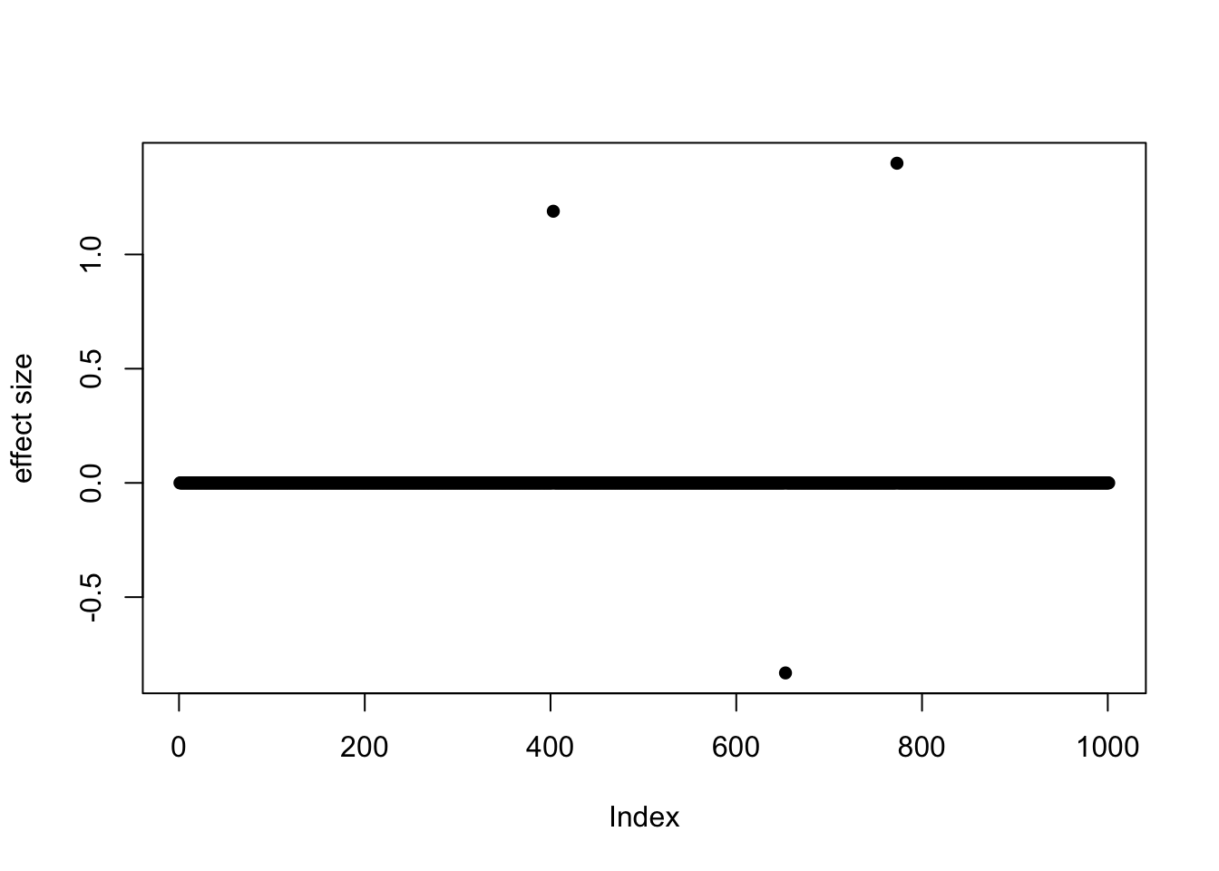
Expand here to see past versions of unnamed-chunk-12-1.png:
| Version | Author | Date |
|---|---|---|
| cd773c5 | zouyuxin | 2018-09-18 |
which(b != 0) ## 403 653 773[1] 403 653 773z_scores = dat$sumstats[1,,] / dat$sumstats[2,,]
z_scores = z_scores[,1]
susie_plot(z_scores, y = "z", b=b)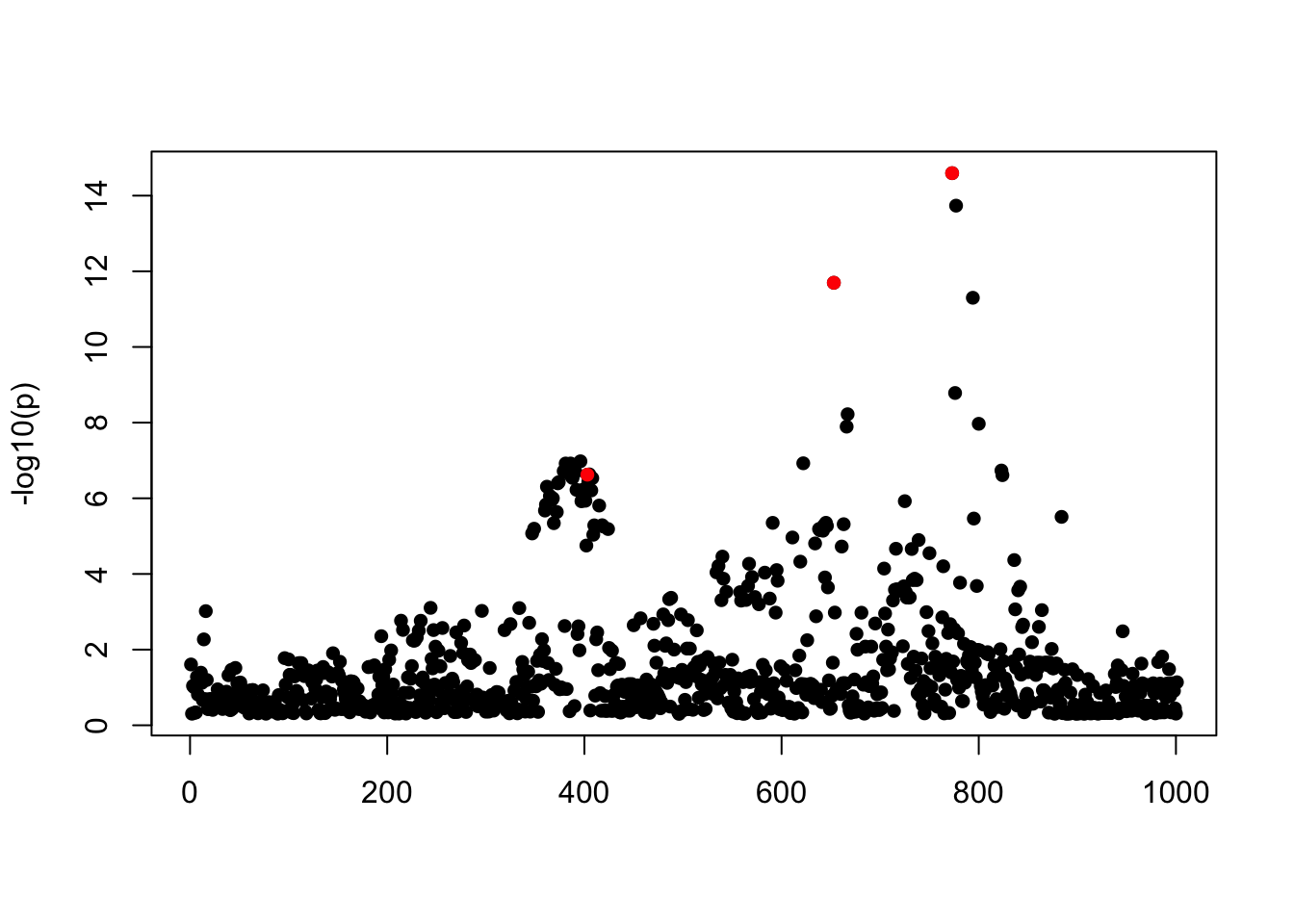
Expand here to see past versions of unnamed-chunk-12-2.png:
| Version | Author | Date |
|---|---|---|
| 73cf69a | zouyuxin | 2018-10-06 |
| cd773c5 | zouyuxin | 2018-09-18 |
SuSiE model with individual level data
fitted = susie(dat$data$X, dat$data$Y[,1],
               L=5,
               estimate_residual_variance = FALSE,
               estimate_prior_variance = FALSE,
               scaled_prior_variance = 0.1,
               tol=1e-3)
sets = susie_get_CS(fitted)
pip = susieR::susie_get_PIP(fitted, sets$cs_index)
susieR::susie_plot(fitted, y='PIP', b=b, main = paste('SuSiE, ', length(sets$cs), 'CS identified'))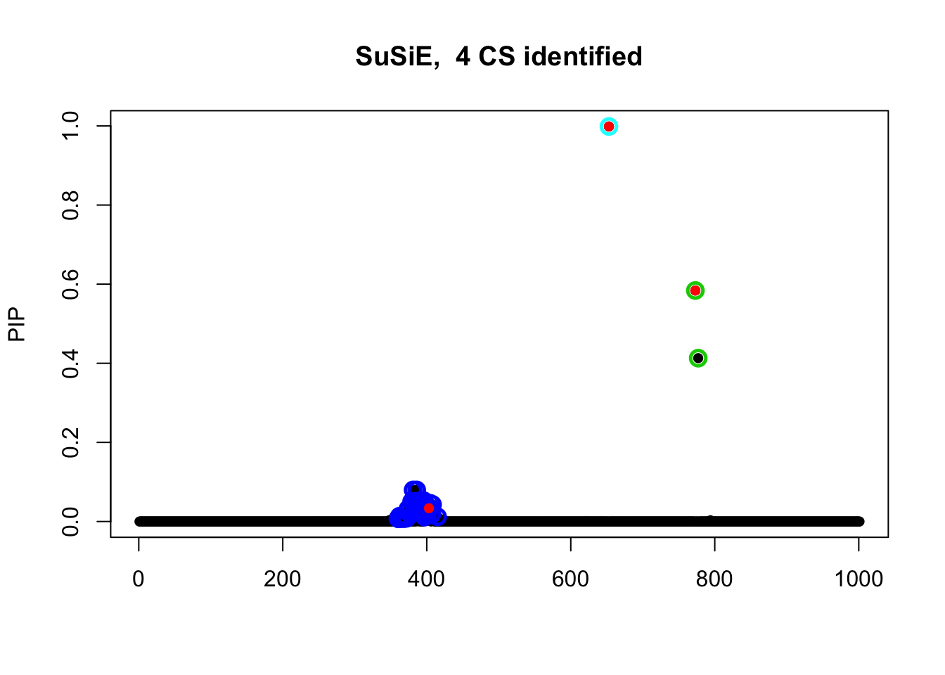
Expand here to see past versions of unnamed-chunk-13-1.png:
| Version | Author | Date |
|---|---|---|
| 73cf69a | zouyuxin | 2018-10-06 |
| cd773c5 | zouyuxin | 2018-09-18 |
SuSiE model using summary stat
n = nrow(dat$data$X)
R = cor(dat$data$X)

R2 = z_scores^2/(z_scores^2 + n-2)
sigma2 = (n-1)*(1-R2)/(n-2)
sXtXz = (n-1)*R
sXtyz = sqrt(n-1) * sqrt(sigma2) * z_scores

fitted_ss = susie_ss(sXtXz, sXtyz,
               L=5, var_y = 1, n = n,
               residual_variance = 1,
               estimate_prior_variance = FALSE,
               scaled_prior_variance = 0.1,
               tol=1e-3, max_iter = 6)

all.equal(fitted$alpha, fitted_ss$alpha)
[1] TRUEsets_ss = susie_get_CS(fitted_ss)
pip_ss = susieR::susie_get_PIP(fitted, sets_ss$cs_index)
susieR::susie_plot(fitted_ss, y='PIP', b=b, main = paste('SuSiE, ', length(sets_ss$cs), 'CS identified'))
Session information
sessionInfo()R version 3.5.1 (2018-07-02)
Platform: x86_64-apple-darwin15.6.0 (64-bit)
Running under: macOS High Sierra 10.13.6
Matrix products: default
BLAS: /Library/Frameworks/R.framework/Versions/3.5/Resources/lib/libRblas.0.dylib
LAPACK: /Library/Frameworks/R.framework/Versions/3.5/Resources/lib/libRlapack.dylib
locale:
[1] en_US.UTF-8/en_US.UTF-8/en_US.UTF-8/C/en_US.UTF-8/en_US.UTF-8
attached base packages:
[1] stats graphics grDevices utils datasets methods base
other attached packages:
[1] susieR_0.4.30.0332
loaded via a namespace (and not attached):
[1] workflowr_1.1.1 Rcpp_0.12.19 matrixStats_0.54.0
[4] lattice_0.20-35 digest_0.6.15 rprojroot_1.3-2
[7] R.methodsS3_1.7.1 grid_3.5.1 backports_1.1.2
[10] git2r_0.23.0 magrittr_1.5 evaluate_0.11
[13] stringi_1.2.4 whisker_0.3-2 R.oo_1.22.0
[16] R.utils_2.6.0 Matrix_1.2-14 rmarkdown_1.10
[19] tools_3.5.1 stringr_1.3.1 yaml_2.2.0
[22] compiler_3.5.1 htmltools_0.3.6 knitr_1.20 This reproducible R Markdown analysis was created with workflowr 1.1.1