Amelia locus 1563
Yuxin Zou
1/18/2021
Last updated: 2021-01-18
Checks: 7 0
Knit directory: Note/
This reproducible R Markdown analysis was created with workflowr (version 1.6.2). The Checks tab describes the reproducibility checks that were applied when the results were created. The Past versions tab lists the development history.
Great! Since the R Markdown file has been committed to the Git repository, you know the exact version of the code that produced these results.
Great job! The global environment was empty. Objects defined in the global environment can affect the analysis in your R Markdown file in unknown ways. For reproduciblity it’s best to always run the code in an empty environment.
The command set.seed(20180529) was run prior to running the code in the R Markdown file. Setting a seed ensures that any results that rely on randomness, e.g. subsampling or permutations, are reproducible.
Great job! Recording the operating system, R version, and package versions is critical for reproducibility.
Nice! There were no cached chunks for this analysis, so you can be confident that you successfully produced the results during this run.
Great job! Using relative paths to the files within your workflowr project makes it easier to run your code on other machines.
Great! You are using Git for version control. Tracking code development and connecting the code version to the results is critical for reproducibility.
The results in this page were generated with repository version 184f6ac. See the Past versions tab to see a history of the changes made to the R Markdown and HTML files.
Note that you need to be careful to ensure that all relevant files for the analysis have been committed to Git prior to generating the results (you can use wflow_publish or wflow_git_commit). workflowr only checks the R Markdown file, but you know if there are other scripts or data files that it depends on. Below is the status of the Git repository when the results were generated:
Ignored files:
    Ignored:    .DS_Store
    Ignored:    .Rhistory
    Ignored:    .Rproj.user/
    Ignored:    analysis/.Rhistory

Untracked files:
    Untracked:  analysis/Li&Stephens.Rmd
    Untracked:  data/locus1563.RDS

Unstaged changes:
    Modified:   analysis/LD_space.Rmd
    Modified:   analysis/bibliography.bib
Note that any generated files, e.g. HTML, png, CSS, etc., are not included in this status report because it is ok for generated content to have uncommitted changes.
These are the previous versions of the repository in which changes were made to the R Markdown (analysis/amelialocus1563.Rmd) and HTML (docs/amelialocus1563.html) files. If you’ve configured a remote Git repository (see ?wflow_git_remote), click on the hyperlinks in the table below to view the files as they were in that past version.
| File | Version | Author | Date | Message |
|---|---|---|---|---|
| Rmd | 184f6ac | zouyuxin | 2021-01-18 | wflow_publish(“analysis/amelialocus1563.Rmd”) |
dat = readRDS('data/locus1563.RDS')
z = dat$gwas$zscore
logp = -log10(pnorm(-abs(z))*2)
R = cor(dat$genotypes)
z_ld_weight = 1/500

# modify R with z
Rmod = cov2cor((1-z_ld_weight)*R + z_ld_weight * tcrossprod(z))
Rmod = (Rmod + t(Rmod))/2
Plot of z scores from GWAS and corresponding p values(the red point is the SNP in CS):
par(mfrow=c(1,2))
plot(z, main='z scores')
points(210, z[210], col='red', pch=16)
plot(logp, ylab='-log10 pvalues', main='-log10 pvalues')
points(210, logp[210], col='red', pch=16)
We reproduce susie_rss result under L=1:
library(susieR)
res = susieR::susie_rss(z, Rmod, L=1)
susie_plot(res, y='PIP')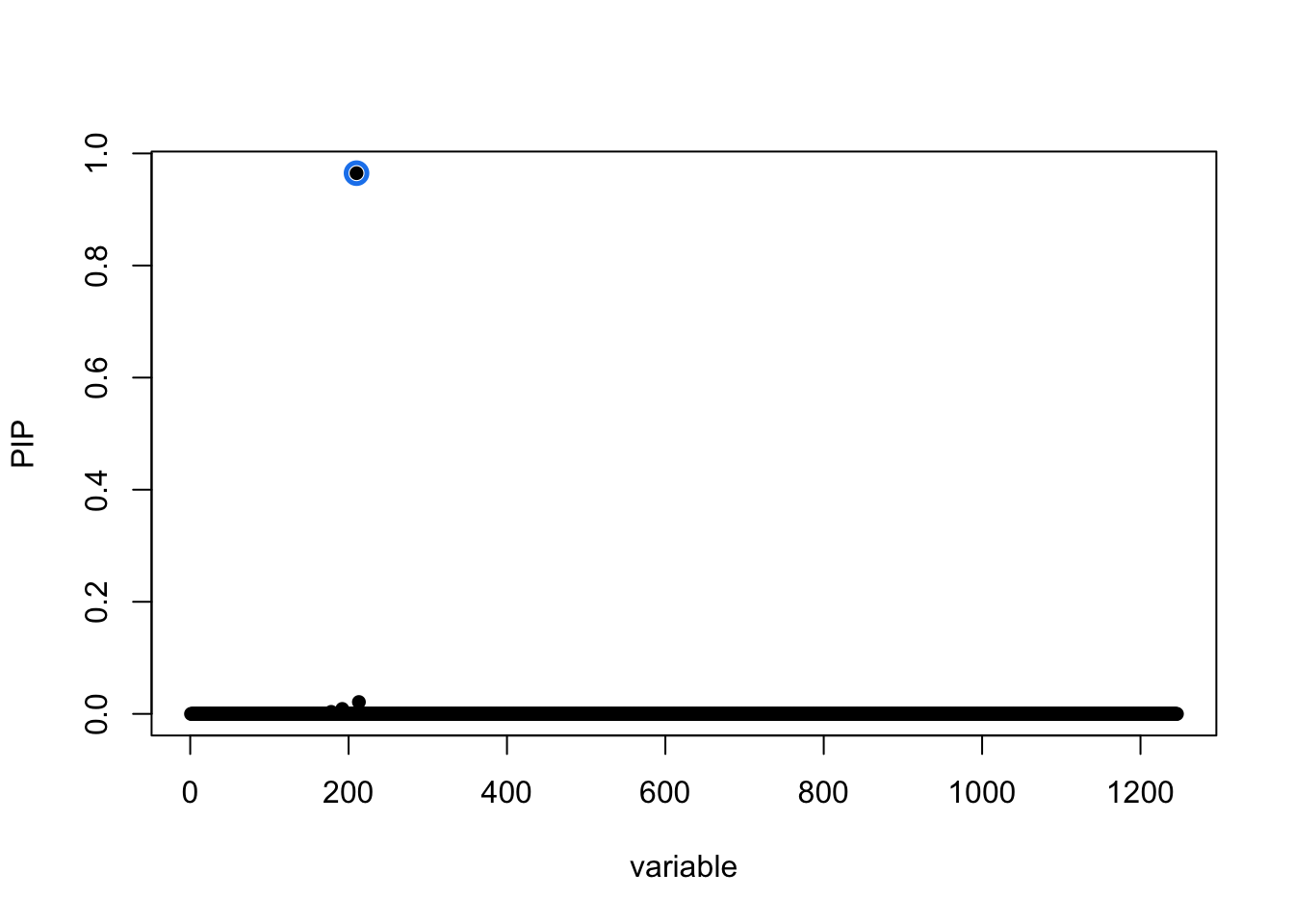 The CS is
res$sets$cs$L1
[1] 210Since the LD matrix is from a reference panel, we used z_ld_weight = 1/500 to adjust LD matrix. The details are in https://stephenslab.github.io/susieR/articles/finemapping_summary_statistics.html#using-ld-from-reference-panel.
The question is why SNP 210 has PIP close to 1 while there are other SNPs in high LD and similar p values. The susie_rss model is based on the projected z scores in the column space of LD.
After projecting z into column space of LD, the z scores are
eigenR = eigen(Rmod, symmetric = T)
eigenR$values[abs(eigenR$values) < 1e-8] = 0

Rhat = eigenR$vectors %*% (eigenR$values * t(eigenR$vectors))
U = eigenR$vectors[,eigenR$values > 0]
UUz = U %*% crossprod(U, z)
par(mfrow=c(1,2))
plot(UUz, main='projected z scores')
points(210, UUz[210], col='red', pch=16)
plot(-log10(pnorm(-abs(UUz))*2), ylab = '-log10 p', main='- log10 pvalues for projected z scores')
points(210, -log10(pnorm(-abs(UUz))*2)[210], col='red', pch=16)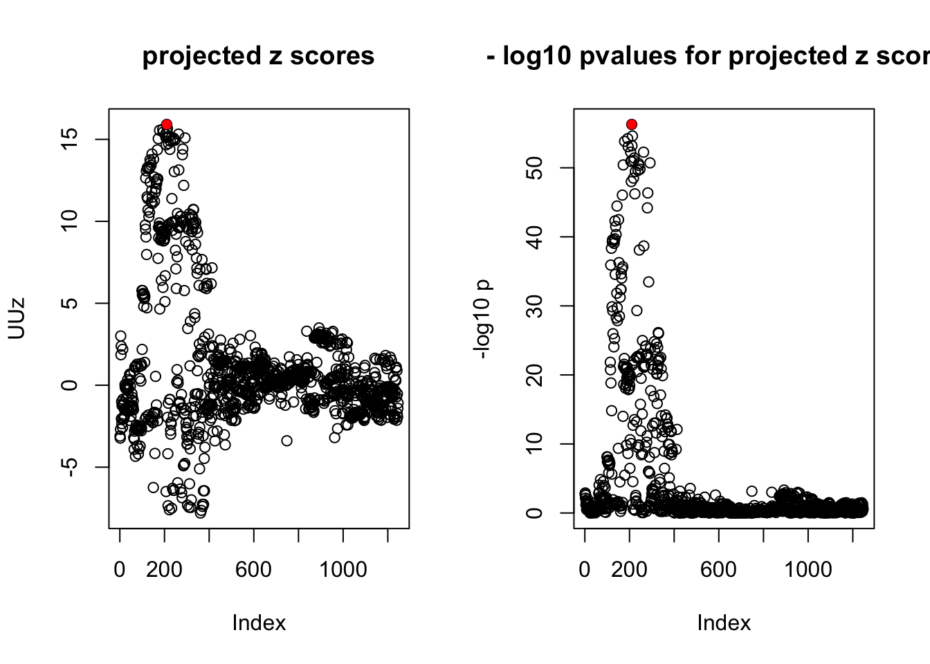 The 210 SNP has the strongest signal. The minimum correlation between the top SNP and the SNPs around (with p values \(< 10^{-50}\)) it is 0.88. There is no SNP in perfect correlation with SNP 210.
With L = 1, the PIP doesn’t depend on LD. The PIP is normalized Bayes Factor and the Bayes Factor is related to the projected z scores, \(BF\propto \exp(0.5* \text{(posterior variance)} * \text{(projected z)}^2)\).
par(mfrow=c(2,2))
plot(UUz^2, ylab = '(projected z)^2', main='(projected z)^2')
points(210, UUz[210]^2, col='red', pch=16)
plot(exp(UUz^2), ylab='exp((projected z)^2)', main = 'exp((projected z)^2)')
points(210, exp(UUz[210]^2), col='red', pch=16)
post_var = 1/(1+1/252)
bf = exp(0.5*post_var*UUz^2)
plot(bf, ylab='BF', main='BF')
points(210, bf[210], col='red', pch=16)
plot(bf/sum(bf), ylab='normalized BF', main='PIP = normalized BF')
points(210, bf[210]/sum(bf), col='red', pch=16)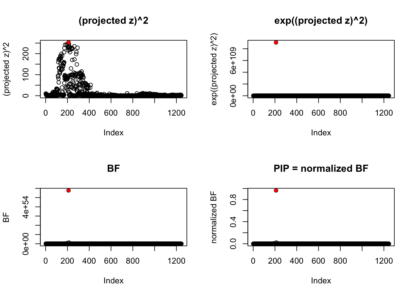 The SNP 210 has PIP close to 1 because it has the strongest z score and there is no SNP in perfect LD with it.
sessionInfo()R version 4.0.3 (2020-10-10)
Platform: x86_64-apple-darwin17.0 (64-bit)
Running under: macOS Big Sur 10.16
Matrix products: default
BLAS: /Library/Frameworks/R.framework/Versions/4.0/Resources/lib/libRblas.dylib
LAPACK: /Library/Frameworks/R.framework/Versions/4.0/Resources/lib/libRlapack.dylib
locale:
[1] en_US.UTF-8/en_US.UTF-8/en_US.UTF-8/C/en_US.UTF-8/en_US.UTF-8
attached base packages:
[1] stats graphics grDevices utils datasets methods base
other attached packages:
[1] susieR_0.9.57 workflowr_1.6.2
loaded via a namespace (and not attached):
[1] Rcpp_1.0.5 plyr_1.8.6 pillar_1.4.7 compiler_4.0.3
[5] later_1.1.0.1 git2r_0.27.1 tools_4.0.3 digest_0.6.27
[9] evaluate_0.14 lifecycle_0.2.0 tibble_3.0.4 gtable_0.3.0
[13] lattice_0.20-41 pkgconfig_2.0.3 rlang_0.4.10 Matrix_1.2-18
[17] rstudioapi_0.13 yaml_2.2.1 xfun_0.19 dplyr_1.0.2
[21] stringr_1.4.0 knitr_1.30 generics_0.1.0 fs_1.5.0
[25] vctrs_0.3.6 tidyselect_1.1.0 rprojroot_2.0.2 grid_4.0.3
[29] reshape_0.8.8 glue_1.4.2 R6_2.5.0 rmarkdown_2.5
[33] purrr_0.3.4 ggplot2_3.3.3 magrittr_2.0.1 whisker_0.4
[37] scales_1.1.1 promises_1.1.1 ellipsis_0.3.1 htmltools_0.5.0
[41] colorspace_2.0-0 httpuv_1.5.4 stringi_1.5.3 munsell_0.5.0
[45] crayon_1.3.4