- Chapter 2 Unconstrained Optimization
- Chapter 3 Line Search Methods
- Step length
- Convergence Theory
- Rate of convergence
- Newton’s Methos with Hessian Modification
- Chapter 4 Trust-Region Methods
- Exact solution
- Approximate solution
- Convergence
- Enhancements
- Chapter 5 Conjugate Gradient Methods
- Linear Conjugate Gradient Method
- Non-Linear Conjugate Gradient Methods
Numerical Optimization
Yuxin Zou
5/2/2020
Last updated: 2020-06-24
Checks: 2 0
Knit directory: Note/
This reproducible R Markdown analysis was created with workflowr (version 1.6.1). The Checks tab describes the reproducibility checks that were applied when the results were created. The Past versions tab lists the development history.
Great! Since the R Markdown file has been committed to the Git repository, you know the exact version of the code that produced these results.
Great! You are using Git for version control. Tracking code development and connecting the code version to the results is critical for reproducibility.
The results in this page were generated with repository version 484483b. See the Past versions tab to see a history of the changes made to the R Markdown and HTML files.
Note that you need to be careful to ensure that all relevant files for the analysis have been committed to Git prior to generating the results (you can use wflow_publish or wflow_git_commit). workflowr only checks the R Markdown file, but you know if there are other scripts or data files that it depends on. Below is the status of the Git repository when the results were generated:
Ignored files:
    Ignored:    .DS_Store
    Ignored:    .Rhistory
    Ignored:    .Rproj.user/
    Ignored:    analysis/.Rhistory

Untracked files:
    Untracked:  analysis/Li&Stephens.Rmd

Unstaged changes:
    Modified:   analysis/bibliography.bib
Note that any generated files, e.g. HTML, png, CSS, etc., are not included in this status report because it is ok for generated content to have uncommitted changes.
These are the previous versions of the repository in which changes were made to the R Markdown (analysis/NumericalOptimization.Rmd) and HTML (docs/NumericalOptimization.html) files. If you’ve configured a remote Git repository (see ?wflow_git_remote), click on the hyperlinks in the table below to view the files as they were in that past version.
| File | Version | Author | Date | Message |
|---|---|---|---|---|
| Rmd | 484483b | zouyuxin | 2020-06-24 | wflow_publish(“analysis/NumericalOptimization.Rmd”) |
| html | def0336 | zouyuxin | 2020-06-17 | Build site. |
| Rmd | 36c9c83 | zouyuxin | 2020-06-17 | wflow_publish(“analysis/NumericalOptimization.Rmd”) |
| html | 5ff4d37 | zouyuxin | 2020-06-17 | Build site. |
| Rmd | 5ad5cde | zouyuxin | 2020-06-17 | wflow_publish(“analysis/NumericalOptimization.Rmd”) |
| html | 29b7bc7 | zouyuxin | 2020-05-20 | Build site. |
| Rmd | d862df4 | zouyuxin | 2020-05-20 | wflow_publish(“analysis/NumericalOptimization.Rmd”) |
| html | 59381e5 | zouyuxin | 2020-05-20 | Build site. |
| Rmd | a84b349 | zouyuxin | 2020-05-20 | wflow_publish(“analysis/NumericalOptimization.Rmd”) |
| html | 2bb2cbb | zouyuxin | 2020-05-15 | Build site. |
| Rmd | 34077d7 | zouyuxin | 2020-05-15 | wflow_publish(“analysis/NumericalOptimization.Rmd”) |
| html | e6dba0f | zouyuxin | 2020-05-15 | Build site. |
| Rmd | 6c98a27 | zouyuxin | 2020-05-15 | wflow_publish(“analysis/NumericalOptimization.Rmd”) |
| html | d25e4b0 | zouyuxin | 2020-05-15 | Build site. |
| Rmd | 9dd586e | zouyuxin | 2020-05-15 | wflow_publish(“analysis/NumericalOptimization.Rmd”) |
| html | c9852b0 | zouyuxin | 2020-05-15 | Build site. |
| Rmd | 4382068 | zouyuxin | 2020-05-15 | wflow_publish(“analysis/NumericalOptimization.Rmd”) |
| html | 760df04 | zouyuxin | 2020-05-03 | Build site. |
| Rmd | 0f786f5 | zouyuxin | 2020-05-03 | wflow_publish(“analysis/NumericalOptimization.Rmd”) |
Notes about book Nocedal and Wright (2006).
Chapter 2 Unconstrained Optimization
A point x⋆ is a local minimizer if there is a neighborhood N of x⋆ such that f(x⋆)≤f(x) for all x∈N.
A point x⋆ is an isolated local minimizer if there is a neighborhood N of x⋆ such that x⋆ is the only local minimizer in N.
While strict local minimizers are not always isolated, it is true that all isolated local minimizers are strict.
Taylor’s Theorem: Suppose that f:Rn→R is continuously differentiable and that p∈Rn. Then we have that f(x+p)=f(x)+∇f(x+tp)⊺ for some t \in (0,1). Moreover, if f is twice continuously differentiable, we have that \nabla f(x+p) = \nabla f(x) + \int_0^1 \nabla^2 f(x+tp)p dt, and that f(x+p) = f(x) + \nabla f(x)^\intercal p + \frac{1}{2} p^\intercal \nabla^2 f(x+tp) p, for some t \in (0,1).
First-Order Necessary Conditions: If x^\star is a local minimizer and f is continuously differentiable in an open neighborhood of x^\star, then \nabla f(x^\star) = 0.
Second-Oder Necessary Conditions: If x^\star is a local minimizer of f and \nabla^2 f exists and is continuous in an open neighborhood of x^\star, then \nabla f(x^\star) = 0 and \nabla^2 f(x^\star) is positive semidefinite.
Second-Oder Sufficient Conditions: Suppose that \nabla^2 f is continuous in an open neighborhood of x^\star and that \nabla f(x^\star) = 0 and \nabla^2 f(x^\star) is positive semidefinite. Then x^\star is a strict local minimizer of f.
Two strategies:
- line search: for direction p_k, \min_{\alpha > 0} f(x_k + \alpha p_k)
Start by fixing the direction p_k and then identifying an appropriate distance.
The steepest descent mehtod is a line search method that moves along p_k = -\nabla f_k at every step.
Newton direction: p_k^N = -(\nabla^2 f_k)^{-1} \nabla f_k. Reliable when f(x_k + p) \approx m_k(p).
Quasi-Newton: In place of the true Hessian \nabla^2 f_k, they use an approximation B_k. By Taylor’s Thm, \nabla f(x+p) = \nabla f(x) + \nabla^2 f(x) p + \int_0^1 [\nabla^2 f(x+tp) - \nabla^2 f(x)]p dt. Let x = x_k, p = x_{k+1} - x_k, then \nabla f_{k+1} = \nabla f_k + \nabla^2 f_k (x_{k+1}-x_{k}) + o(\| x_{k+1} - x_{k} \|). We choose B_{k+1} s.t. B_{k+1} s_k = y_k, \quad s_k = x_{k+1} - x_k, \quad y_k = \nabla f_{k+1} - \nabla f_{k}
Symmetric-rank-one (SR1) formula: B_{k+1} = B_{k} + \frac{(y_k - B_k s_k)(y_k - B_k s_k)^\intercal}{(y_k - B_k s_k)^\intercal s_k} BFGS formula: B_{k+1} = B_{k} - \frac{B_k s_k s_k^\intercal B_k}{s_k^\intercal B_k s_k} + \frac{y_k y_k^\intercal}{ y_k^\intercal s_k }
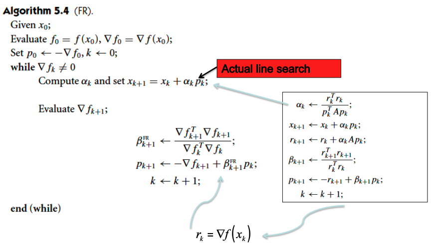
Nonlinear conjugate gradient methods: p_k = -\nabla f(x_k) + \beta_k p_{k-1}, where \beta_k is a scalar that ensures that p_k and p_{k-1} are conjugate.
- trust region: the information gathered about f is used to construct a model function m_k whose behavior near the current point x_k is similar to that of the actual objective function f. We find the candidate steo p by approxiamtely solving the following subproblem: \min_p m_k(x_k + p), \text{where } x_k + p \text{ lies inside the trust region.} The model m_k is usually defined to be a quadratic function of the form m_k(x_k+p) = f_k + p^\intercal \nabla f_k + \frac{1}{2} p^\intercal B_k p.
First choose a maximum distance and then seek a direction and step that attain the best improvement possible subject to this distance constraint.
When B_k = 0, the problem becomes \min_{p} f_k + p^\intercal \nabla f_k s.t. \|p\|_2 \leq \Delta_k, which has solution p_k = -\Delta_k \nabla f_k /\|\nabla f_k\| (same as steepest descent step).
Chapter 3 Line Search Methods
step length: \alpha_k, direction: p_k x_{k+1} = x_{k} + \alpha_k p_k The search direction often has the form p_k = -B_k^{-1} \nabla f_k, B_k \text{ symmetrix and nonsingular matrix}, so p_k^\intercal \nabla f_k = -\nabla f_k^\intercal B_k^{-1} \nabla f_k < 0 if B_k is positive definite.
Steepest descent method: B_k = I
Newton’s method: B_k = \nabla^2 f(x_k)
Step length
The Wolfe Conditions
- Sufficient descent
f(x_k + \alpha p_k) \leq f(x_k) + c_1 \alpha \nabla f_k^\intercal p_k, c_1 \in (0,1)
In practice, c_1 = 10^{-4}.
- Curvature condition
\nabla f(x_k + \alpha_k p_k)^\intercal p_k \geq c_2 \nabla f_k^\intercal p_k, c_2 \in (c_1, 1)
Lemma 3.1
Suppose that f: \mathbb{R}^n \rightarrow \mathbb{R} is continuously differentiable. Let p_k be a descent direction at x_k, and asusme that f is bounded below along the ray \{x_k + \alpha p_k | \alpha > 0\}. Then if 0 < c_1 < c_2 < 1, there exist intervals of step lengths satisfying the Wolfe conditions.
Goldstein Condition (Newton-type method)
f(x_k) + (1-c) \alpha_k \nabla f_k^\intercal p_k \leq f(x_k + \alpha_k p_k) \leq f(x_k) + c \alpha_k \nabla f_k^\intercal p_k, 0 < c < 1/2
Backtracking
Algorithm: Choose \bar{\alpha} > 0, \rho \in (0,1), c \in (0,1); Set \alpha \leftarrow \bar{\alpha};
repeat until f(x_k + \alpha p_k) \leq f(x_k) + c \alpha \nabla f_k^\intercal p_k: \alpha \leftarrow \rho \alpha;
For Newton and quasi-Newton: \bar{\alpha} = 1.
Convergence Theory
Zoutendijk Theorem: If the Wolfe conditions hold, then we must have \cos^2 \theta_k \|\nabla f_k\|^2 \rightarrow 0 \quad \cos \theta_k = \frac{-\nabla f_k^\intercal p_k}{\|\nabla f_k\| \|p_k\|}
If the angle is bounded amway from 90^\circ, then \|\nabla f_k\| \rightarrow 0. (globally convergent)
Consider Newton-like method: x_{k+1} = x_k + \alpha_k p_k; \quad p_k = -B_k^{-1} \nabla f_k B_k is bounded and uniformly positive definite: \|B_k\| \|B_k^{-1}\| \leq M Then \cos \theta_k \geq 1/M and \|\nabla f_k\| \rightarrow 0.
Rate of convergence
Steepest descent
Suppose f(x) = \frac{1}{2} x^\intercal Q x - b^\intercal x, the gradient is \nabla f(x) = Qx - b. For line search, \alpha_k = \frac{\nabla f_k^\intercal \nabla f_k}{\nabla f_k^\intercal Q \nabla f_k} Using weighted norm \|x\|_Q^2 = x^\intercal Q x, we have \|x_{k+1} - x^\star\|_Q^2 = \{ 1- \frac{(\nabla f_k^\intercal \nabla f_k)^2}{(\nabla f_k^\intercal Q \nabla f_k)(\nabla f_k^\intercal Q^{-1} \nabla f_k)} \} \|x_{k} - x^\star\|_Q^2
For strongly convex quadratic function, \|x_{k+1} - x^\star\|_Q^2 \leq (\frac{\lambda_n - \lambda_1}{\lambda_n + \lambda_1})^2 \|x_{k} - x^\star\|_Q^2, where 0 < \lambda_1 \leq \lambda_2 \leq \cdots \leq \lambda_n are eigenvalues of Q.
Newton’s Method p_k^N = -\nabla^2 f_k^{-1} \nabla f_k
If the starting point x_0 is sufficiently close to x^\star, the sequence of iterates converges to x^\star;
the rate of convergence of \{x_k\} is quadratic;
the sequence of gradient norms \{\|\nabla f_k\|\} converges quadratically to 0.
Quasi-Newton Method p_k = -B_k^{-1} \nabla f_k
Newton’s Methos with Hessian Modification
If the problem is not convex, far away from the solution, Newton’s direction is not necessarity a descent direction.
General framework:
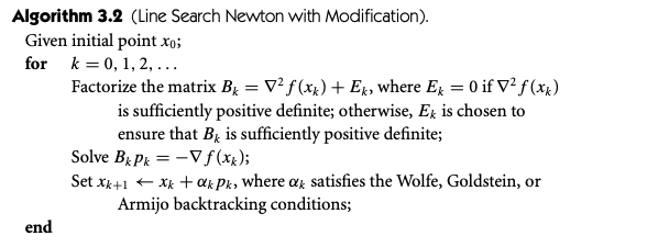
Modified Symmetric Indefinite Factorization
PAP^\intercal = LBL^\intercal A symmetric, L unit lower triangular, B bloack diagonal with blocks of dim 1 or 2, P permutation matrix. B has same number of positive and negative eigenvalues as A.
Modified version: P(A + E)P^\intercal = L(B+F)L^\intercal, where E = P^\intercal LFL^\intercal P.
Chapter 4 Trust-Region Methods
Trust-region methods define a region around the current iterate within which they trust the model to be an adequate representation of the objective function, and then choose the step to be the approximate minimizer of the model in this region. In effect, they choose the direction and length of the step simultaneously. The direction of the step changes whenever the size of the trust region is altered.
The model function m_k used at each iterate x_k is quadratic, m_k is based on the Taylor-series expansion of f around x_k, m_k(p) = f_k + g_k^\intercal p + \frac{1}{2} p^\intercal B_k p. (g_k = \nabla f(x_k))
Trust region Newton method: B_k = \nabla^2 f(x_k).
We seek a solution of the subproblem \min_{p \in \mathbb{R}^n} m_k(p) = f_k + g_k^\intercal p + \frac{1}{2} p^\intercal B_k p \quad s.t. \quad \|p\| \leq \Delta_k where \Delta_k > 0 is the trust-region radius.
Exact solution
p^\star statisfies
(B + \lambda I) p^\star = -g \quad \text{ for some } \lambda \geq 0
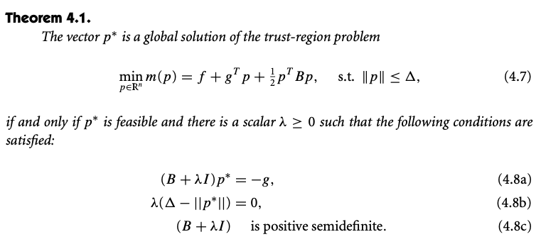
Find \lambda > 0 s.t.
p(\lambda) = -(B + \lambda I)^{-1} g \quad \|p(\lambda)\| = \Delta
Using eigendecomposition of B = Q\Lambda Q^\intercal (\lambda_1 \leq \lambda_2 \leq \cdots \leq \lambda_n), we have
p(\lambda) = -\sum_{j=1}^n \frac{q_j^\intercal g}{\lambda_j + \lambda} q_j, \quad \|p(\lambda)\|^2 = \sum_{j=1}^n \frac{(q_j^\intercal g)^2}{(\lambda_j + \lambda)^2}
Note that: \lim_{\lambda \rightarrow\infty} \|p(\lambda)\| = 0. Good case: q_j^\intercal g \neq 0, then \lim_{\lambda \rightarrow -\lambda_j} \|p(\lambda)\| = \infty, so there must be a solution. The practical algorithm: 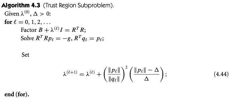 It needs to with large enough \lambda.
Hard case: q_j^\intercal g = 0
\lambda = -\lambda_1, p = -\sum_{j: \lambda_j \neq \lambda_1}^n \frac{q_j^\intercal g}{\lambda_j + \lambda} q_j. We set p(\tau) = -\sum_{j: \lambda_j \neq \lambda_1}^n \frac{q_j^\intercal g}{\lambda_j + \lambda} q_j + \tau q_1. There always exist \tau s.t. \|p(\tau)\| = \Delta.
Approximate solution
- Cauchy point
It’s easier to solve linear model: l(p) = f + g^\intercal p. Solve TR linear model
p^s = \arg \min_{\|p\|\leq \Delta} f + g^\intercal p \Rightarrow p^s = -\frac{\Delta}{\|g\|}g.
The Cauchy point, \tau = \arg \min_{\|\tau p^s\| \leq \Delta} m(\tau p^s). 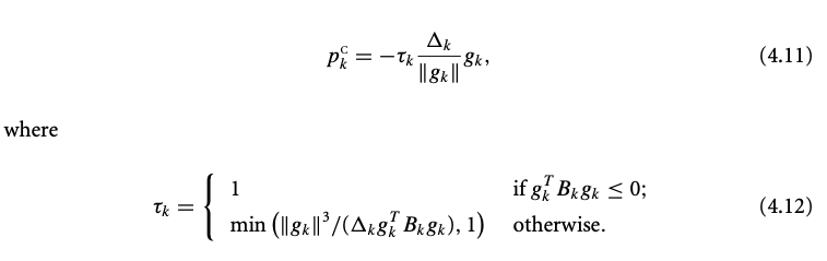
Dogleg method (B positive definite)
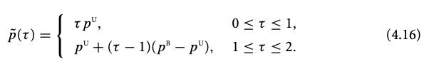 p^U is the Cauchy point,
p^U = -\frac{g^\intercal g}{g^\intercal B g} g.
p^B is the Newton’s direction,
p^B = - B^{-1} g
p^U is the Cauchy point,
p^U = -\frac{g^\intercal g}{g^\intercal B g} g.
p^B is the Newton’s direction,
p^B = - B^{-1} g
Two-dimensional subspace minimization
Use the linear combination of g and B^{-1}g, \min_p m(p) = f + g^\intercal p + \frac{1}{2}p^\intercal B p \quad s.t. \|p\|\leq \Delta, p \in span[g, B^{-1}g] If B is indefinite, we can find \alpha s.t. B + \alpha I is pd. If \|(B+\alpha I )^{-1}g\| \leq \Delta, p = -(B+\alpha I)^{-1} g + v, s.t. v^\intercal (B+\alpha I)^{-1} g \leq 0. Otherwise, p \in span[g, (B+\alpha I )^{-1}g]
Convergence
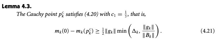
Algorithmic requirement : improvement in the MODEL is bounded below by some coercive function of the gradient.
m(0) - m(p) \geq c_1 \|g\| \min(\Delta, \frac{\|g\|}{\|B\|}), c_1 \in (0,1]
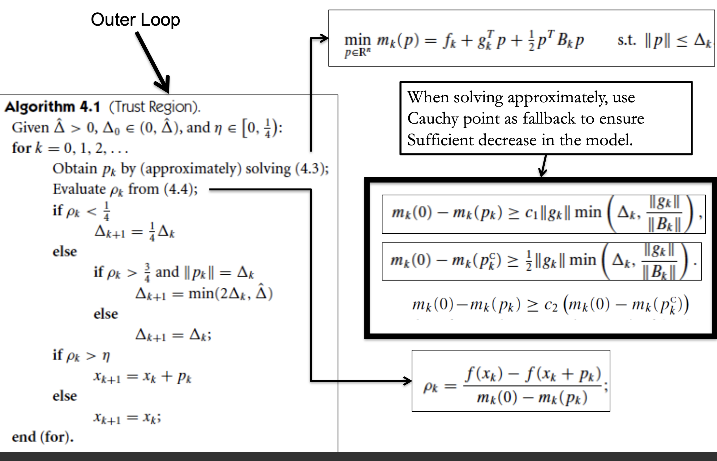
When \eta = 0, \lim \inf_{k \rightarrow \infty} \|g_k\| = 0.
When \eta > 0, \lim_{k \rightarrow \infty} g_k = 0.
Enhancements
- Bad scaled problem – elliptical TR:
\min m(p) = f + g^\intercal p + \frac{1}{2} p^\intercal B p \quad \|Dp\| \leq \Delta D is a diagonal matrix with positive diagonal elements.
- Other norms: \|p\|_1 \leq \Delta or \|p\|_\infty \leq \Delta.
This is useful in bound constrained optimization: \min f(x), \quad s.t. x\geq 0 \min m(p) = f + g^\intercal p + \frac{1}{2} p^\intercal B p \quad s.t. x+p\geq 0, \|p\| \leq \Delta When the \infty-norm is used, the feasible resion is simply the rectangular box x + p \geq 0, \quad p \geq -\Delta 1, \quad p \leq \Delta 1
Chapter 5 Conjugate Gradient Methods
Most useful techniques for solving large linear systems of equations.
Linear Conjugate Gradient Method
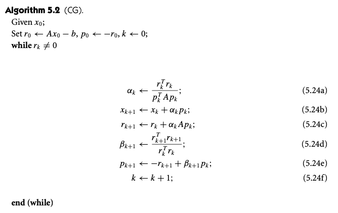
Conjugate gradient method is an iterative method for solving a linear system of equations Ax = b, A \text{ is } n \times n \text{ symmetric positive definite }. This is equivalent as \min \phi(x) = \frac{1}{2} x^\intercal A x - b^\intercal x. The gradient of \phi is the residual of the linear system, \nabla \phi(x) = Ax - b = r(x)
Definition: nonzero vectors \{p_0, p_1, \cdots, p_l\} is conjugate with respect to the synnetric positive definite matrix A if p_i^\intercal A p_j = 0, i\neq j, which also implies linearly independent.
- Conjugate direction method
Given a starting point x_0 \in \mathbb{R}^n and a set of conjugate directions S = \{p_0, p_1,\cdots, p_{n-1}\}, x_{k+1} = x_{k} + \alpha_k p_k, where \alpha_k is teh one-dimensional minimizer of \phi along x_k + \alpha p_k, \alpha_k = -\frac{r_k^\intercal p_k}{p_k^\intercal A p_k}
- Conjugate gradient method
The space of the search directions should coincide with the space of the residuuals. S_k = \{r_0, r_1, \cdots, r_{k-1}\}.
If A has only r distinct eigenvalues, then the CG iteration will terminate at the solution in at most r iterations.
Preconditioning
Transform the linear system to improve the eigenvalue distribution of A. \hat{x} = C x The problem becomes (C^{-\intercal} A C^{-1}) \hat{x} = C^{-\intercal} b.
Non-Linear Conjugate Gradient Methods
The Fletcher-Reeves Method
Nocedal, Jorge, and Stephen Wright. 2006. Numerical Optimization. Springer Science & Business Media.