Different Cov
Yuxin Zou
12/10/2018
Last updated: 2018-12-19
workflowr checks: (Click a bullet for more information)-
✔ R Markdown file: up-to-date
Great! Since the R Markdown file has been committed to the Git repository, you know the exact version of the code that produced these results.
-
✔ Environment: empty
Great job! The global environment was empty. Objects defined in the global environment can affect the analysis in your R Markdown file in unknown ways. For reproduciblity it’s best to always run the code in an empty environment.
-
✔ Seed:
set.seed(20180529)The command
set.seed(20180529)was run prior to running the code in the R Markdown file. Setting a seed ensures that any results that rely on randomness, e.g. subsampling or permutations, are reproducible. -
✔ Session information: recorded
Great job! Recording the operating system, R version, and package versions is critical for reproducibility.
-
Great! You are using Git for version control. Tracking code development and connecting the code version to the results is critical for reproducibility. The version displayed above was the version of the Git repository at the time these results were generated.✔ Repository version: ced6304
Note that you need to be careful to ensure that all relevant files for the analysis have been committed to Git prior to generating the results (you can usewflow_publishorwflow_git_commit). workflowr only checks the R Markdown file, but you know if there are other scripts or data files that it depends on. Below is the status of the Git repository when the results were generated:
Note that any generated files, e.g. HTML, png, CSS, etc., are not included in this status report because it is ok for generated content to have uncommitted changes.Ignored files: Ignored: .DS_Store Ignored: .Rhistory Ignored: .Rproj.user/ Ignored: analysis/.Rhistory Ignored: docs/.DS_Store Ignored: docs/figure/Test.Rmd/ Untracked files: Untracked: analysis/DifferentCovModelR50.Rmd Untracked: analysis/MASH_est_Cor.Rmd Untracked: analysis/MashEstCorProblem.Rmd Untracked: analysis/MashMedian.Rmd Untracked: analysis/mashMean.Rmd Untracked: code/DifferentCov.R Untracked: code/EstCorV.R Untracked: code/generateDataV.R Untracked: code/summary.R Untracked: docs/Estimate_Null_Cor_New.pdf Untracked: docs/Estimate_Null_Cor_Old.pdf Untracked: output/MASH.result.1.rds Untracked: output/MASH.result.10.rds Untracked: output/MASH.result.2.rds Untracked: output/MASH.result.3.rds Untracked: output/MASH.result.4.rds Untracked: output/MASH.result.5.rds Untracked: output/MASH.result.6.rds Untracked: output/MASH.result.7.rds Untracked: output/MASH.result.8.rds Untracked: output/MASH.result.9.rds Unstaged changes: Modified: analysis/susieProblem2.Rmd
Expand here to see past versions:
| File | Version | Author | Date | Message |
|---|---|---|---|---|
| Rmd | ced6304 | zouyuxin | 2018-12-19 | wflow_publish(“analysis/DifferentCovModel.Rmd”) |
| html | d144bac | zouyuxin | 2018-12-12 | Build site. |
| Rmd | 3c5a13d | zouyuxin | 2018-12-12 | wflow_publish(“analysis/DifferentCovModel.Rmd”) |
| html | 7ff2647 | zouyuxin | 2018-12-11 | Build site. |
| Rmd | 3a32721 | zouyuxin | 2018-12-11 | wflow_publish(“analysis/DifferentCovModel.Rmd”) |
| html | 8ba1a51 | zouyuxin | 2018-12-11 | Build site. |
| Rmd | 42b495f | zouyuxin | 2018-12-11 | wflow_publish(“analysis/DifferentCovModel.Rmd”) |
knitr::read_chunk("code/DifferentCov.R")library(plyr)
DifferentCov = function(data, Ulist,
gridmult= sqrt(2),
control = list(),
pi_thresh = 1e-10,
outputlevel = 2){
grid = mashr:::autoselect_grid(data, gridmult)
Ulist = mashr:::normalize_Ulist(Ulist)
prior = "uniform"
L = length(Ulist)
grid.full = c(0, grid)
xUlist.null = rep(Ulist, length(grid.full))
xUlist = mashr:::expand_cov(Ulist,grid.full,FALSE)
xUlist.full = Map("+", xUlist.null, xUlist)
lm = calc_relative_lik_matrix(data,xUlist.full)
prior = mashr:::set_prior(ncol(lm$loglik_matrix),prior)
pi_s = mashr:::optimize_pi(exp(lm$loglik_matrix),prior=prior,optmethod='mixSQP', control=control)
which.comp = (pi_s > pi_thresh)
posterior_weights = mashr:::compute_posterior_weights(pi_s,exp(lm$loglik_matrix))
if (outputlevel > 1) {
xUlistinv = rep(lapply(xUlist.null[1:L], function(U) solve(U)), length(grid.full))
posterior_cov = mashr:::expand_cov(Ulist,sqrt((grid.full^2)/(1+grid.full^2)),FALSE)
posterior_matrices = compute_posterior_matrices(data,xUlistinv, posterior_cov, posterior_weights)
} else {
posterior_matrices = NULL
}
vloglik = mashr:::compute_vloglik_from_matrix_and_pi(pi_s,lm, data$Shat_alpha)
loglik = sum(vloglik)
null_loglik = compute_null_loglik_from_matrix(pi_s, lm, data$Shat_alpha, L)
alt_loglik = compute_alt_loglik_from_matrix_and_pi(pi_s, lm, data$Shat_alpha, L)
# results
fitted_g = list(pi=pi_s, Ulist=Ulist, grid=grid.full, usepointmass=FALSE)
m=list(result = posterior_matrices,
loglik = loglik, vloglik = vloglik,
null_loglik = null_loglik,
alt_loglik = alt_loglik,
fitted_g = fitted_g,
posterior_weights = posterior_weights,
alpha=data$alpha)
#for debugging
if(outputlevel==4){m = c(m,list(lm=lm))}
return(m)
}
#' Compute vector of null loglikelihoods from a matrix of log-likelihoods
#' @param lm the results of a likelihood matrix calculation from \code{calc_relative_lik_matrix}
#' whose first column corresponds to null
#' @param Shat_alpha matrix of Shat^alpha
compute_null_loglik_from_matrix = function(pi_s, lm,Shat_alpha, L){
return(log(exp(lm$loglik_matrix[,1:L,drop=FALSE]) %*% (pi_s[1:L]/(1-sum(pi_s[-c(1:L)])))) +lm$lfactors-rowSums(log(Shat_alpha)))
}
#' Compute vector of alternative loglikelihoods from a matrix of log-likelihoods and fitted pi
#' @param pi_s the vector of mixture proportions, with first element corresponding to null
#' @param lm the results of a likelihood matrix calculation from \code{calc_relative_lik_matrix}
#' whose first column corresponds to null
#' @param Shat_alpha matrix of Shat^alpha
compute_alt_loglik_from_matrix_and_pi = function(pi_s,lm,Shat_alpha,L){
return(log(exp(lm$loglik_matrix[,-c(1:L),drop=FALSE]) %*% (pi_s[-c(1:L)]/(1-sum(pi_s[1:L]))))+lm$lfactors-rowSums(log(Shat_alpha)))
}
calc_lik_matrix_common_cov = function(data, Ulist, log = FALSE){
res <- laply(Ulist,function(U)
dmvnorm(x = data$Bhat,sigma = U,log = log))
dimnames(res) = NULL # just to make result identical to the non-common-cov version
return(t(res))
}
calc_lik_matrix <- function (data, Ulist, log = FALSE) {
res <- calc_lik_matrix_common_cov(data,Ulist,log)
if (nrow(res) == 1)
res <- matrix(res)
if (ncol(res) > 1)
colnames(res) <- names(Ulist)
# Give a warning if any columns have -Inf likelihoods.
rows <- which(apply(res,2,function (x) any(is.infinite(x))))
if (length(rows) > 0)
warning(paste("Some mixture components result in non-finite likelihoods,",
"either\n","due to numerical underflow/overflow,",
"or due to invalid covariance matrices",
paste(rows,collapse=", "),
"\n"))
return(res)
}
calc_relative_lik_matrix <-
function (data, Ulist) {
# Compute the J x P matrix of conditional log-likelihoods.
matrix_llik <- calc_lik_matrix(data,Ulist,log = TRUE)
# Avoid numerical issues (overflow or underflow) by subtracting the
# largest entry in each row.
lfactors <- apply(matrix_llik,1,max)
matrix_llik <- matrix_llik - lfactors
return(list(loglik_matrix = matrix_llik,
lfactors = lfactors))
}
posterior_mean <- function(bhat, Vinv, U1){
return(U1 %*% (Vinv %*% bhat))
}
#' @title posterior_mean_matrix
#' @param Bhat J by R matrix of observations
#' @param Vinv R x R inverse covariance matrix for the likelihood
#' @param U1 R x R posterior covariance matrix, computed using posterior_cov
#' @return R vector of posterior mean
#' @description Computes posterior mean under multivariate normal model for each row of matrix Bhat.
#' Note that if bhat is N_R(b,V) and b is N_R(0,U) then b|bhat N_R(mu1,U1).
#' This function returns a matrix with jth row equal to mu1(bhat) for bhat= Bhat[j,].
posterior_mean_matrix <- function(Bhat, Vinv, U1){
return(Bhat %*% (Vinv %*% U1))
}
compute_posterior_matrices <-
function (data, Ulistinv, posterior_cov, posterior_weights) {
R = mashr:::n_conditions(data)
# keep data dimension names
effect_names = rownames(data$Bhat)
condition_names = colnames(data$Bhat)
posterior_matrices = compute_posterior_matrices_general_R(data, Ulistinv, posterior_cov, posterior_weights)
# Set dimension names
for (i in names(posterior_matrices)) {
if (length(dim(posterior_matrices[[i]])) == 2) {
colnames(posterior_matrices[[i]]) <- condition_names
rownames(posterior_matrices[[i]]) <- effect_names
}
}
if (length(dim(posterior_matrices$PosteriorCov)) == 3)
dimnames(posterior_matrices$PosteriorCov) <- list(condition_names, condition_names, effect_names)
return(posterior_matrices)
}
compute_posterior_matrices_general_R=function(data,Ulistinv, posterior_cov,posterior_weights){
R=mashr:::n_conditions(data)
J=mashr:::n_effects(data)
P=length(posterior_cov)
# allocate arrays for returned results
res_post_mean=array(NA,dim=c(J,R))
res_post_mean2 = array(NA,dim=c(J,R)) #mean squared value
res_post_zero=array(NA,dim=c(J,R))
res_post_neg=array(NA,dim=c(J,R))
# allocate arrays for temporary calculations
post_mean=array(NA,dim=c(P,R))
post_mean2 = array(NA,dim=c(P,R)) #mean squared value
post_zero=array(NA,dim=c(P,R))
post_neg=array(NA,dim=c(P,R))
U1 = posterior_cov
for(j in 1:J){
bhat=as.vector(t(data$Bhat[j,]))##turn j into a R x 1 vector
for(p in 1:P){
mu1 <- as.array(posterior_mean(bhat, Ulistinv[[p]], U1[[p]]))
# Transformation for mu
muA <- (mu1 * data$Shat_alpha[j,])
# Transformation for Cov
covU = data$Shat_alpha[j,] * t(data$Shat_alpha[j,] * U1[[p]])
pvar = covU
post_var = pmax(0,diag(pvar)) # Q vector posterior variance
post_mean[p,]= muA
post_mean2[p,] = muA^2 + post_var #post_var is the posterior variance
post_neg[p,] = ifelse(post_var==0,0,pnorm(0,mean=muA,sqrt(post_var),lower.tail=T))
post_zero[p,] = ifelse(post_var==0,1,0)
}
res_post_mean[j,] = posterior_weights[j,] %*% post_mean
res_post_mean2[j,] = posterior_weights[j,] %*% post_mean2
res_post_zero[j,] = posterior_weights[j,] %*% post_zero
res_post_neg[j,] = posterior_weights[j,] %*% post_neg
}
res_post_sd = sqrt(res_post_mean2 - res_post_mean^2)
res_lfsr = compute_lfsr(res_post_neg,res_post_zero)
posterior_matrices = list(PosteriorMean = res_post_mean,
PosteriorSD = res_post_sd,
lfdr = res_post_zero,
NegativeProb = res_post_neg,
lfsr = res_lfsr)
return(posterior_matrices)
}ROC.table = function(data, model){
sign.test = data*model$result$PosteriorMean
thresh.seq = seq(0, 1, by=0.005)[-1]
m.seq = matrix(0,length(thresh.seq), 2)
colnames(m.seq) = c('TPR', 'FPR')
for(t in 1:length(thresh.seq)){
m.seq[t,] = c(sum(sign.test>0 & model$result$lfsr <= thresh.seq[t])/sum(data!=0),
sum(data==0 & model$result$lfsr <=thresh.seq[t])/sum(data==0))
}
return(m.seq)
}
library(knitr)
library(kableExtra)
library(mvtnorm)
library(mashr)Loading required package: ashr
Attaching package: 'mashr'The following object is masked _by_ '.GlobalEnv':
compute_posterior_matricesThe model is on z scores \[ \hat{\mathbf{z}}_j \sim \sum_{k=1}^{K} \sum_{l=1}^{L} \pi_{kl} N(0, (1+\omega_{l})U_{k}) \] We can also write the model as \[ \hat{\mathbf{z}}_j | \mathbf{z}_j, \gamma_{j}=(k, l) \sim N(\mathbf{z}_j, U_{k}) \\ \mathbf{z}_j|\gamma_{j}=(k, l) \sim N(0, \omega_{l}U_{k}) \\ P(\gamma_{j}=(l,k)) = \pi_{kl} \] We assume \(U_k\) are all invertible. Under the null, \(\omega_l = 0\).
Simulate Simple 1
I simulate null data with common error.
\[ \hat{\mathbf{z}}_j | \mathbf{z}_j \sim N(\mathbf{z}_j, I) \\ \mathbf{z}_j = \delta_0 \]
set.seed(1)
n = 10000; p = 2
B = matrix(0,n,p)
Bhat = rmvnorm(n, sigma = diag(p))
data = mash_set_data(Bhat=Bhat, Shat=1)

Ulist = cov_canonical(data, cov_methods = c('identity', 'simple_het'))

model = DifferentCov(data, Ulist)
m.model = mash(data, Ulist, verbose = FALSE)
loglike = c(get_loglik(model), get_loglik(m.model))
sig = c(length(get_significant_results(model)), length(get_significant_results(m.model)))
rrmse = c(sqrt(mean((B - model$result$PosteriorMean)^2)/mean((B - Bhat)^2)), sqrt(mean((B - m.model$result$PosteriorMean)^2)/mean((B - Bhat)^2)))
tmp = cbind(loglike, sig, rrmse)
colnames(tmp) = c('logliklihood', '#sig', 'RRMSE')
rownames(tmp) = c('new', 'mash')
tmp %>% kable() %>% kable_styling()| logliklihood | #sig | RRMSE | |
|---|---|---|---|
| new | -28410.56 | 0 | 0.0031717 |
| mash | -28410.60 | 0 | 0.0000000 |
par(mfrow=c(1,2))
barplot(get_estimated_pi(model, dimension = 'grid'), las=2, names.arg = round(model$fitted_g$grid, 2), main='new')
barplot(get_estimated_pi(model), las=2, main='new')
Expand here to see past versions of unnamed-chunk-5-1.png:
| Version | Author | Date |
|---|---|---|
| d144bac | zouyuxin | 2018-12-12 |
| 7ff2647 | zouyuxin | 2018-12-11 |
| 8ba1a51 | zouyuxin | 2018-12-11 |
barplot(get_estimated_pi(m.model), las=2, main='mash')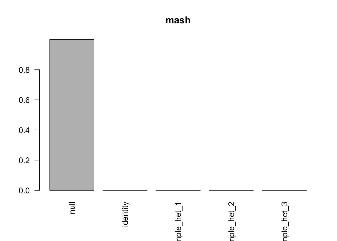
Expand here to see past versions of unnamed-chunk-6-1.png:
| Version | Author | Date |
|---|---|---|
| 7ff2647 | zouyuxin | 2018-12-11 |
Simulate Simple 2
I simulate null data with different errors. \[ \hat{\mathbf{z}}_j | \mathbf{z}_j \sim \frac{1}{2}N(\mathbf{z}_j, I) + \frac{1}{2}N(\mathbf{z}_j,\left( \begin{matrix} 1 & 0.75 \\ 0.75 & 1\end{matrix} \right)) \\ \mathbf{z}_j = \delta_0 \]
set.seed(1)
B = matrix(0,n,p)
Bhat1 = rmvnorm(n/2, sigma = diag(p))
V = matrix(0.75, p,p); diag(V) = 1
Bhat2 = rmvnorm(n/2, sigma = V)
Bhat = rbind(Bhat1, Bhat2)
V.true = array(0,dim=c(p,p,n))
V.true[,,1:(n/2)] = diag(p)
V.true[,,(n/2 + 1):n] = V
data = mash_set_data(Bhat=Bhat, Shat=1)

Ulist = cov_canonical(data, cov_methods = c('identity', 'simple_het'))

model = DifferentCov(data, Ulist)

Vhat = estimate_null_correlation(data, Ulist)
m.model.current = Vhat$mash.model

data.true = mash_update_data(data, V = V.true)
m.model.true = mash(data.true, Ulist, algorithm.version = 'R', verbose=FALSE)
loglike = c(get_loglik(model), get_loglik(m.model.current), get_loglik(m.model.true))
sig = c(length(get_significant_results(model)), length(get_significant_results(m.model.current)), length(get_significant_results(m.model.true)))
rrmse = c(sqrt(mean((B - model$result$PosteriorMean)^2)/mean((B - Bhat)^2)), sqrt(mean((B - m.model.current$result$PosteriorMean)^2)/mean((B - Bhat)^2)), sqrt(mean((B - m.model.true$result$PosteriorMean)^2)/mean((B - Bhat)^2)))
tmp = cbind(loglike, sig, rrmse)
colnames(tmp) = c('logliklihood', '#sig', 'RRMSE')
rownames(tmp) = c('new', 'mash current', 'mash true')
tmp %>% kable() %>% kable_styling()| logliklihood | #sig | RRMSE | |
|---|---|---|---|
| new | -27449.11 | 0 | 0.0070456 |
| mash current | -27585.51 | 2 | 0.0816107 |
| mash true | -26343.82 | 0 | 0.0021181 |
par(mfrow=c(1,2))
barplot(get_estimated_pi(model, dimension = 'grid'), las=2, names.arg = round(model$fitted_g$grid, 2), main='new')
barplot(get_estimated_pi(model), las=2, main='new')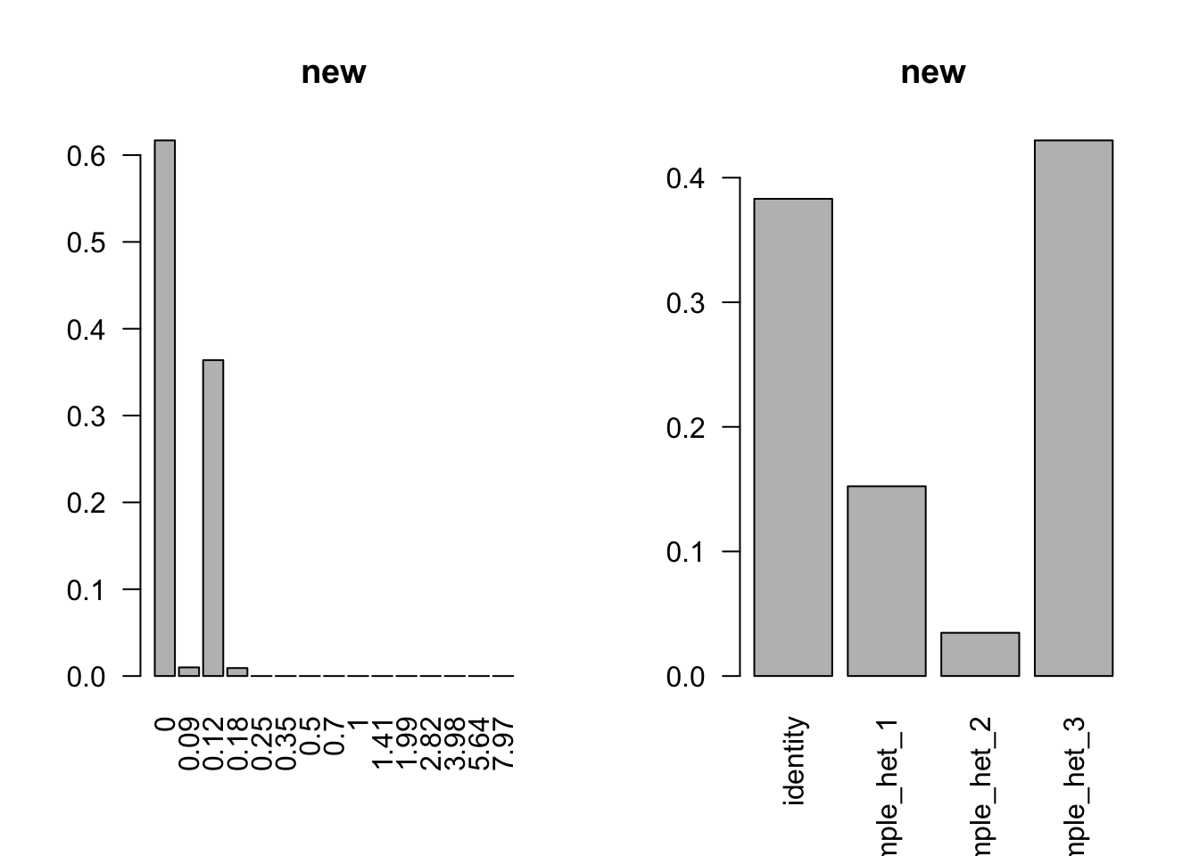
Expand here to see past versions of unnamed-chunk-9-1.png:
| Version | Author | Date |
|---|---|---|
| d144bac | zouyuxin | 2018-12-12 |
| 7ff2647 | zouyuxin | 2018-12-11 |
| 8ba1a51 | zouyuxin | 2018-12-11 |
barplot(get_estimated_pi(m.model.current), las=2, main='mash current')
Expand here to see past versions of unnamed-chunk-10-1.png:
| Version | Author | Date |
|---|---|---|
| 7ff2647 | zouyuxin | 2018-12-11 |
| 8ba1a51 | zouyuxin | 2018-12-11 |
barplot(get_estimated_pi(m.model.true), las=2, main='mash true')
Expand here to see past versions of unnamed-chunk-11-1.png:
| Version | Author | Date |
|---|---|---|
| 7ff2647 | zouyuxin | 2018-12-11 |
Simulate with signal 1
I simulate data with signal, but common error. \[ \hat{\mathbf{z}}_j | \mathbf{z}_j \sim N(\mathbf{z}_j, I) \\ \mathbf{z}_j \sim \frac{1}{2}\delta_0 + \frac{1}{2} N(0, I) \]
set.seed(1)
B1 = matrix(0,n/2,p)
B2 = matrix(rnorm((n/2)*p),n/2,p)
B = rbind(B1, B2)
Ehat = rmvnorm(n, sigma = diag(p))
Bhat = B + Ehat

data = mash_set_data(Bhat=Bhat, Shat=1)

Ulist = cov_canonical(data, cov_methods = c('identity', 'simple_het'))

model = DifferentCov(data, Ulist)
m.model = mash(data, Ulist, verbose = FALSE)
loglike = c(get_loglik(model), get_loglik(m.model))
sig = c(length(get_significant_results(model)), length(get_significant_results(m.model)))
fd = c(sum(get_significant_results(model)<=5000), sum(get_significant_results(m.model)<=5000))
rrmse = c(sqrt(mean((B - model$result$PosteriorMean)^2)/mean((B - Bhat)^2)), sqrt(mean((B - m.model$result$PosteriorMean)^2)/mean((B - Bhat)^2)))
tmp = cbind(loglike, sig, fd, rrmse)
colnames(tmp) = c('logliklihood', '#sig', 'false pos','RRMSE')
rownames(tmp) = c('new', 'mash')
tmp %>% kable() %>% kable_styling()| logliklihood | #sig | false pos | RRMSE | |
|---|---|---|---|---|
| new | -32407.42 | 122 | 1 | 0.5716567 |
| mash | -32407.63 | 121 | 1 | 0.5715801 |
roc.seq = ROC.table(B, model)
plot(roc.seq[,'FPR'], roc.seq[,'TPR'], type='l', xlab = 'FPR', ylab='TPR',
       main=paste0(' True Pos vs False Pos'), cex=1.5, lwd = 1.5, col = 'cyan')
roc.seq = ROC.table(B, m.model)
lines(roc.seq[,'FPR'], roc.seq[,'TPR'], col='purple', lwd = 1.5)
legend('bottomright', c('new','mash'), col=c('cyan','purple'),
           lty=c(1,1), lwd=c(1.5,1.5))
Expand here to see past versions of unnamed-chunk-14-1.png:
| Version | Author | Date |
|---|---|---|
| d144bac | zouyuxin | 2018-12-12 |
| 7ff2647 | zouyuxin | 2018-12-11 |
| 8ba1a51 | zouyuxin | 2018-12-11 |
par(mfrow=c(1,2))
barplot(get_estimated_pi(model, dimension = 'grid'), las=2, names.arg = round(model$fitted_g$grid, 2), main='new')
barplot(get_estimated_pi(model), las=2, main='new')
Expand here to see past versions of unnamed-chunk-15-1.png:
| Version | Author | Date |
|---|---|---|
| d144bac | zouyuxin | 2018-12-12 |
| 7ff2647 | zouyuxin | 2018-12-11 |
| 8ba1a51 | zouyuxin | 2018-12-11 |
barplot(get_estimated_pi(m.model), las=2, main='mash')
Expand here to see past versions of unnamed-chunk-16-1.png:
| Version | Author | Date |
|---|---|---|
| 7ff2647 | zouyuxin | 2018-12-11 |
Simulate with signal 2
I simulate data with signal, but different error.
\[ \hat{\mathbf{z}}_j \sim \frac{1}{2} N(0, I) + \frac{1}{2}N(0, \left( \begin{matrix} 1 & 0.75 \\ 0.75 & 1\end{matrix} \right) + \left( \begin{matrix} 1 & 0.75 \\ 0.75 & 1\end{matrix} \right)) \\ \mathbf{z}_j \sim \frac{1}{2}\delta_0 + \frac{1}{2} N(0, \left( \begin{matrix} 1 & 0.75 \\ 0.75 & 1\end{matrix} \right)) \]
set.seed(1)
B1 = matrix(0,n/2,p)
B2 = rmvnorm(n/2, sigma = V)
B = rbind(B1, B2)

Ehat1 = rmvnorm(n/2, sigma = diag(p))
Ehat2 = rmvnorm(n/2, sigma = V)
Ehat = rbind(Ehat1, Ehat2)

V.true = array(0,dim=c(p,p,n))
V.true[,,1:(n/2)] = diag(p)
V.true[,,(n/2 + 1):n] = V

# V.random = array(0, dim=c(p,p,n))
# ind = sample(1:n, n/2)
# V.random[,,ind] = V
# V.random[,,-ind] = diag(p)

# Ehat = matrix(0, n, p)
# Ehat[ind,] = rmvnorm(n/2, sigma = V)
# Ehat[-ind,] = rmvnorm(n/2, sigma = diag(p))

Bhat = B + Ehat

data = mash_set_data(Bhat=Bhat, Shat=1)

Ulist = cov_canonical(data, cov_methods = c('identity', 'simple_het'))

model = DifferentCov(data, Ulist)

Vhat = estimate_null_correlation(data, Ulist)
m.model.current = Vhat$mash.model

data.true = mash_update_data(data, V = V.true)
m.model.true = mash(data.true, Ulist, algorithm.version = 'R', verbose = FALSE)
loglike = c(get_loglik(model), get_loglik(m.model.current), get_loglik(m.model.true))
sig = c(length(get_significant_results(model)), length(get_significant_results(m.model.current)), length(get_significant_results(m.model.true)))
fd = c(sum(get_significant_results(model)<=5000), sum(get_significant_results(m.model.current)<=5000), sum(get_significant_results(m.model.true)<=5000))
rrmse = c(sqrt(mean((B - model$result$PosteriorMean)^2)/mean((B - Bhat)^2)), sqrt(mean((B - m.model.current$result$PosteriorMean)^2)/mean((B - Bhat)^2)), sqrt(mean((B - m.model.true$result$PosteriorMean)^2)/mean((B - Bhat)^2)))
tmp = cbind(loglike, sig, fd, rrmse)
colnames(tmp) = c('logliklihood', '#sig', 'false pos','RRMSE')
rownames(tmp) = c('new', 'mash current', 'mash true')
tmp %>% kable() %>% kable_styling()| logliklihood | #sig | false pos | RRMSE | |
|---|---|---|---|---|
| new | -30834.78 | 340 | 0 | 0.5563476 |
| mash current | -30935.62 | 138 | 1 | 0.5727592 |
| mash true | -30282.03 | 184 | 3 | 0.5824576 |
roc.seq = ROC.table(B, model)
plot(roc.seq[,'FPR'], roc.seq[,'TPR'], type='l', xlab = 'FPR', ylab='TPR',
       main=paste0(' True Pos vs False Pos'), cex=1.5, lwd = 1.5, col = 'cyan')
roc.seq = ROC.table(B, m.model.current)
lines(roc.seq[,'FPR'], roc.seq[,'TPR'], col='purple', lwd = 1.5)
roc.seq = ROC.table(B, m.model.true)
lines(roc.seq[,'FPR'], roc.seq[,'TPR'], col='red', lwd = 1.5)
legend('bottomright', c('new','mash current', 'mash true'), col=c('cyan','purple', 'red'),
           lty=c(1,1,1), lwd=c(1.5,1.5, 1.5))
Expand here to see past versions of unnamed-chunk-19-1.png:
| Version | Author | Date |
|---|---|---|
| d144bac | zouyuxin | 2018-12-12 |
| 7ff2647 | zouyuxin | 2018-12-11 |
| 8ba1a51 | zouyuxin | 2018-12-11 |
par(mfrow=c(1,2))
barplot(get_estimated_pi(model, dimension = 'grid'), las=2, names.arg = round(model$fitted_g$grid, 2), main='new')
barplot(get_estimated_pi(model), las=2, main='new')
Expand here to see past versions of unnamed-chunk-20-1.png:
| Version | Author | Date |
|---|---|---|
| d144bac | zouyuxin | 2018-12-12 |
| 7ff2647 | zouyuxin | 2018-12-11 |
| 8ba1a51 | zouyuxin | 2018-12-11 |
barplot(get_estimated_pi(m.model.current), las=2, main='mash current')
Expand here to see past versions of unnamed-chunk-21-1.png:
| Version | Author | Date |
|---|---|---|
| 7ff2647 | zouyuxin | 2018-12-11 |
| 8ba1a51 | zouyuxin | 2018-12-11 |
barplot(get_estimated_pi(m.model.true), las=2, main='mash true')
Expand here to see past versions of unnamed-chunk-22-1.png:
| Version | Author | Date |
|---|---|---|
| 7ff2647 | zouyuxin | 2018-12-11 |
Session information
sessionInfo()R version 3.5.1 (2018-07-02)
Platform: x86_64-apple-darwin15.6.0 (64-bit)
Running under: macOS 10.14.2
Matrix products: default
BLAS: /Library/Frameworks/R.framework/Versions/3.5/Resources/lib/libRblas.0.dylib
LAPACK: /Library/Frameworks/R.framework/Versions/3.5/Resources/lib/libRlapack.dylib
locale:
[1] en_US.UTF-8/en_US.UTF-8/en_US.UTF-8/C/en_US.UTF-8/en_US.UTF-8
attached base packages:
[1] stats graphics grDevices utils datasets methods base
other attached packages:
[1] mashr_0.2.19.0555 ashr_2.2-23 mvtnorm_1.0-8 kableExtra_0.9.0
[5] knitr_1.20 plyr_1.8.4
loaded via a namespace (and not attached):
[1] lattice_0.20-35 Rmosek_8.0.69 colorspace_1.3-2
[4] htmltools_0.3.6 viridisLite_0.3.0 yaml_2.2.0
[7] rlang_0.3.0.1 R.oo_1.22.0 mixsqp_0.1-92
[10] pillar_1.3.0 R.utils_2.7.0 REBayes_1.3
[13] foreach_1.4.4 stringr_1.3.1 munsell_0.5.0
[16] workflowr_1.1.1 rvest_0.3.2 R.methodsS3_1.7.1
[19] codetools_0.2-15 evaluate_0.12 doParallel_1.0.14
[22] pscl_1.5.2 parallel_3.5.1 highr_0.7
[25] Rcpp_1.0.0 readr_1.1.1 scales_1.0.0
[28] backports_1.1.2 rmeta_3.0 truncnorm_1.0-8
[31] abind_1.4-5 hms_0.4.2 digest_0.6.18
[34] stringi_1.2.4 grid_3.5.1 rprojroot_1.3-2
[37] tools_3.5.1 magrittr_1.5 tibble_1.4.2
[40] crayon_1.3.4 whisker_0.3-2 pkgconfig_2.0.2
[43] MASS_7.3-50 Matrix_1.2-14 SQUAREM_2017.10-1
[46] xml2_1.2.0 assertthat_0.2.0 rmarkdown_1.10
[49] httr_1.3.1 rstudioapi_0.8 iterators_1.0.10
[52] R6_2.3.0 git2r_0.23.0 compiler_3.5.1 This reproducible R Markdown analysis was created with workflowr 1.1.1